Lecture 05: Math Operators and Functions
DATA 351: Data Management with SQL
January 26, 2026
Math Operators and Functions
SQL as a Calculator
PostgreSQL can do math! Let’s start simple:
| ?column? |
|---|
| 4 |
No table needed. SQL evaluates the expression and returns the result.
Basic Math Operators
| Operator | Operation | Example | Result |
|---|---|---|---|
+ |
Addition | 5 + 3 |
8 |
- |
Subtraction | 10 - 4 |
6 |
* |
Multiplication | 6 * 7 |
42 |
/ |
Division | 15 / 4 |
3 |
% |
Modulo (remainder) | 15 % 4 |
3 |
Wait, what? 👀
15 / 4 = 3? d Yes! Integer division truncates. 🤯
Integer Division Trap
Note
Rule: If both operands are integers, result is integer.
Make at least one operand a decimal to get decimal results.
Hands-On: Math with Employee Data
Calculate annual bonus (10% of salary):
| full_name | salary_usd | annual_bonus |
|---|---|---|
| Michael Scott | 75000.00 | 7500.0000 |
| Dwight Schrute | 62000.00 | 6200.0000 |
| Pam Beesly | 42000.00 | 4200.0000 |
Calculating Percent Change
The formula: ((new - old) / old) * 100
Example: If salary goes from $50,000 to $55,000:
| pct_increase |
|---|
| 10.0 |
A 10% raise. (Nice!)
Hands-On: Salary Per Year of Experience
How much does each employee earn per year of experience?
| full_name | salary_usd | years_experience | salary_per_year |
|---|---|---|---|
| Pam Beesly | 42000.00 | 8 | 5250.00 |
| Jim Halpert | 61000.00 | 10 | 6100.00 |
| Dwight Schrute | 62000.00 | 12 | 5166.67 |
The ROUND() Function
ROUND(value, decimal_places) rounds to specified precision:
Note
Always ROUND money calculations for clean output!
The ABS() Function
ABS() returns the absolute value (distance from zero):
Using ABS()
Use case: Finding differences regardless of direction:
Hands-On: Distance from Average Salary
Let’s find how far each employee’s salary is from $55,000:
| full_name | salary_usd | difference | absolute_difference |
|---|---|---|---|
| Michael Scott | 75000.00 | 20000.00 | 20000.00 |
| Pam Beesly | 42000.00 | -13000.00 | 13000.00 |
| Dwight Schrute | 62000.00 | 7000.00 | 7000.00 |
Exponents and Roots
| Function | Description | Example | Result |
|---|---|---|---|
^ |
Exponentiation | 2 ^ 3 |
8 |
\|/ |
Square root | \|/ 16 |
4 |
\|\|/ |
Cube root | \|\|/ 27 |
3 |
SQRT() |
Square root (function) | SQRT(16) |
4 |
Exercise: Calculate Commission
Sales employees have a commission rate. Calculate their potential commission on a $10,000 sale:
Hint: Commission = sale_amount * commission_rate
Take 2 minutes.
Exercise Solution: Commission Calculation
| full_name | commission_rate | commission_on_10k |
|---|---|---|
| Dwight Schrute | 0.08 | 800.00 |
| Jim Halpert | 0.07 | 700.00 |
| Stanley Hudson | 0.05 | 500.00 |
Dwight’s higher rate reflects his #1 salesman status. Obviously.
Aggregate Functions
What Are Aggregate Functions?
Aggregate functions compute a single result from multiple rows.
The Big Five Aggregates
| Function | Description | Example |
|---|---|---|
SUM() |
Total of all values | Total payroll |
AVG() |
Average (mean) | Average salary |
COUNT() |
Number of rows | How many employees |
MIN() |
Smallest value | Lowest salary |
MAX() |
Largest value | Highest salary |
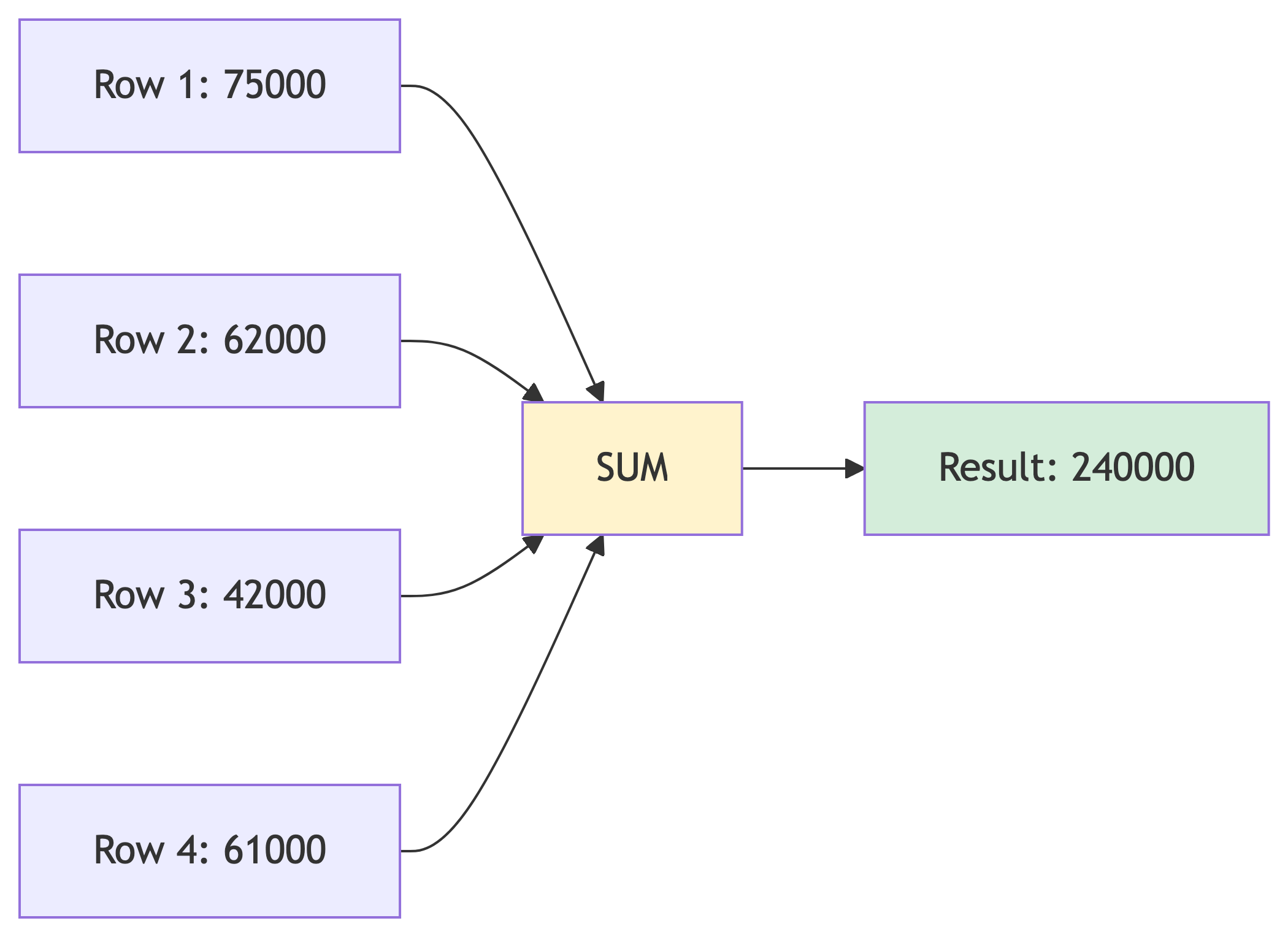
SUM(): Total Values
What is our total payroll?
| total_payroll |
|---|
| 452000.00 |
We spend $452,000 on salaries. (Michael probably thinks he deserves half.)
AVG(): Calculate the Mean
What is the average salary?
| avg_salary |
|---|
| 56500.000000 |
That is a lot of decimal places. Let’s fix that:
| avg_salary |
|---|
| 56500.00 |
COUNT(): How Many?
Three ways to count:
| count(*) | count(commission) | count(distinct dept) |
|---|---|---|
| 8 | 3 | 4 |
Only 3 employees have commission rates!
MIN() and MAX(): The Extremes
Salary range:
| lowest_salary | highest_salary | salary_range |
|---|---|---|
| 42000.00 | 75000.00 | 33000.00 |
Pam makes the least, Michael makes the most. Shocking.
Combining Multiple Aggregates
You can calculate several aggregates in one query:
| num_employees | total_payroll | avg_salary | min_salary | max_salary |
|---|---|---|---|---|
| 8 | 452000.00 | 56500.00 | 42000.00 | 75000.00 |
GROUP BY: Aggregates by Category
What if we want average salary BY DEPARTMENT?
| department | num_employees | avg_salary |
|---|---|---|
| Management | 1 | 75000.00 |
| Sales | 3 | 60333.33 |
| Accounting | 3 | 51333.33 |
| Reception | 1 | 42000.00 |
How GROUP BY Works
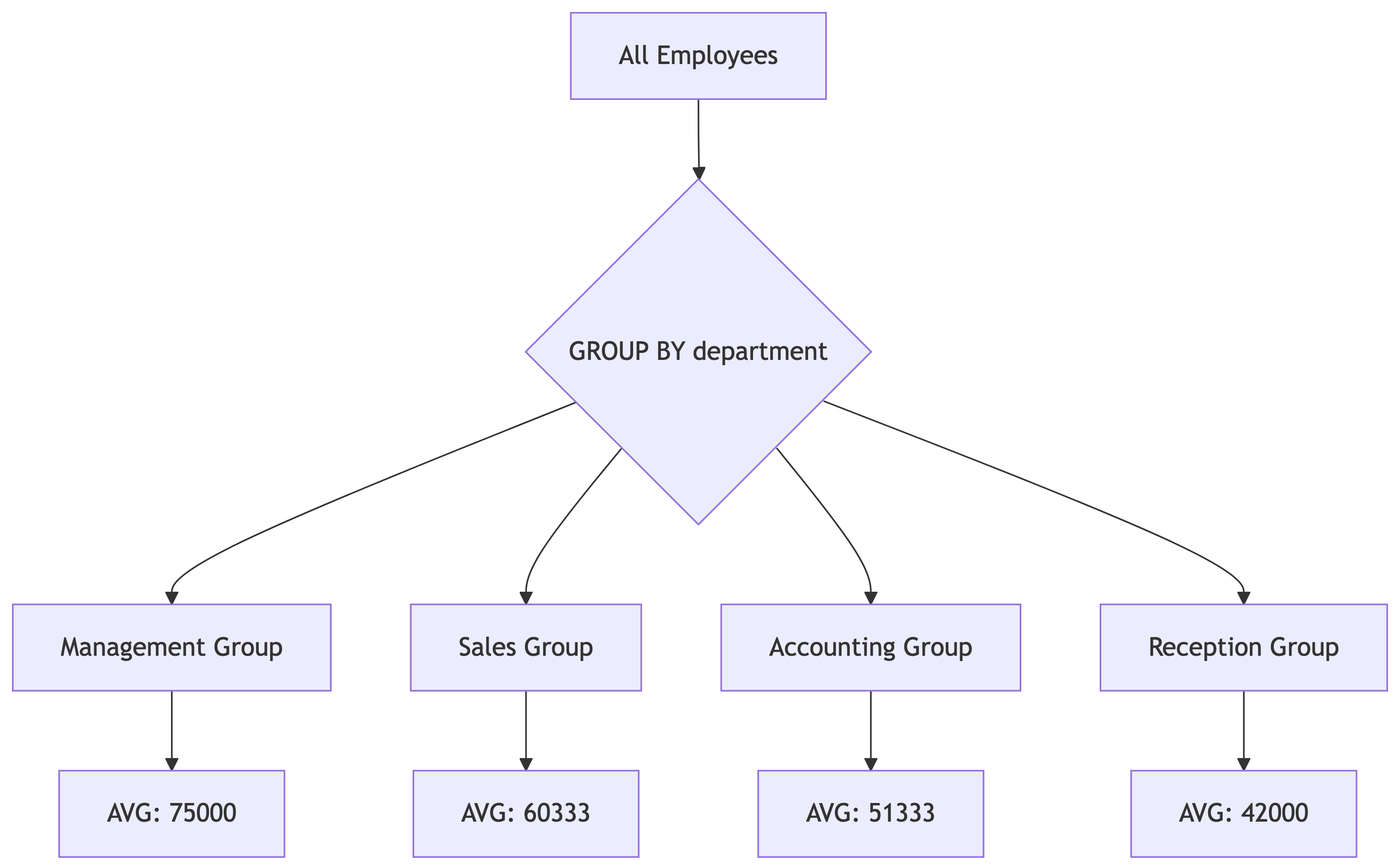
GROUP BY splits data into buckets, then aggregates each bucket separately.
HAVING: Filter After Grouping
Show only departments with more than 1 employee:
| department | num_employees | avg_salary |
|---|---|---|
| Sales | 3 | 60333.33 |
| Accounting | 3 | 51333.33 |
WHERE filters rows BEFORE grouping. HAVING filters AFTER grouping.
Exercise: Department Analysis
Write a query that shows for each department:
- Department name
- Number of employees
- Total salary expense
- Average performance rating (rounded to 1 decimal)
Only include departments where average performance rating > 3.5
Take 4 minutes.
Exercise Solution
| department | num_employees | total_salary | avg_rating |
|---|---|---|---|
| Accounting | 3 | 154000.00 | 3.8 |
| Sales | 3 | 181000.00 | 3.6 |
Management and Reception did not make the cut!
10 Minute Break
When we return: Statistical functions and percentiles!
Up next: Finding the median (and why it matters more than average).
Part 3: Statistics and Percentiles
The Problem with Averages
Pop quiz: A company has 5 employees with these salaries:
$40,000, $42,000, $45,000, $48,000, $500,000
What is the average salary?
Is $135,000 a good representation of “typical” salary? No!
The CEO’s salary skews the average dramatically.
Median: The Middle Value
The median is the middle value when data is sorted.
$40,000, $42,000, $45,000, $48,000, $500,000
The median is $45,000, which better represents “typical.”
Tip
When to use which:
- Mean (average): Data is normally distributed, no outliers
- Median: Data is skewed or has outliers
Finding Median with percentile_cont()
PostgreSQL does not have a built-in MEDIAN() function, but we can use:
| median_salary |
|---|
| 55000 |
The 0.5 means “50th percentile” which is the median.
The WITHIN GROUP Syntax
Let’s break this down:
| Part | Meaning |
|---|---|
percentile_cont(0.5) |
Find the 50th percentile (median) |
WITHIN GROUP |
Required syntax for ordered-set aggregates |
ORDER BY salary_usd |
Which column to calculate percentile on |
Hands-On: Median vs Average
Compare median and average for our employee salaries:
| mean_salary | median_salary |
|---|---|
| 56500.00 | 55000 |
Pretty close! Our data does not have extreme outliers.
What is a Percentile?
A percentile tells you what percentage of values fall below a point.
- 25th percentile: 25% of values are below this
- 50th percentile: 50% are below (the median)
- 75th percentile: 75% are below this
- 90th percentile: 90% are below this
If you score in the 90th percentile on a test, you beat 90% of test-takers.
Calculating Quartiles
Quartiles divide data into four equal parts:
| q1 | q2_median | q3 |
|---|---|---|
| 49000 | 55000 | 61250 |
Using Arrays for Multiple Percentiles
Instead of separate function calls, use an array:
| quartiles |
|---|
| {49000,55000,61250} |
The result is an array. Curly braces indicate array values.
percentile_cont vs percentile_disc
Two versions exist:
| Function | Behavior | Best For |
|---|---|---|
percentile_cont |
Interpolates between values | Continuous data |
percentile_disc |
Returns actual value from data | Discrete data |
Tip
For salaries, percentile_cont is usually more appropriate.
Exercise: Salary Percentile Analysis
Write a query that shows:
- The 10th percentile salary (low end)
- The median salary
- The 90th percentile salary (high end)
Use a single percentile_cont call with an array.
Take 2 minutes.
Exercise Solution
| salary_percentiles |
|---|
| {43400,55000,69550} |
Interpretation:
- 10% of employees make less than $43,400
- 50% make less than $55,000 (median)
- 90% make less than $69,550
Date Arithmetic
Working with Dates in PostgreSQL
PostgreSQL makes date math intuitive:
| days_between |
|---|
| 365 |
Subtracting dates gives you the number of days between them.
Hands-On: Calculate Tenure
How long has each employee been with the company?
| full_name | hire_date | today | days_employed |
|---|---|---|---|
| Stanley Hudson | 2004-11-20 | 2026-01-19 | 7730 |
| Michael Scott | 2005-03-24 | 2026-01-19 | 7606 |
| Jim Halpert | 2005-10-05 | 2026-01-19 | 7411 |
EXTRACT(): Pull Parts from Dates
EXTRACT(part FROM date) gets specific components:
| full_name | hire_date | hire_year | hire_month | day_of_week |
|---|---|---|---|---|
| Michael Scott | 2005-03-24 | 2005 | 3 | 4 |
DOW = Day of Week (0=Sunday, 1=Monday, etc.)
DATE_PART(): Alternative Syntax
DATE_PART('part', date) does the same thing:
| full_name | hire_year | hire_quarter |
|---|---|---|
| Michael Scott | 2005 | 1 |
| Angela Martin | 2006 | 3 |
Use whichever syntax you prefer. They are equivalent.
Grouping by Date Parts
How many employees were hired each year?
| hire_year | num_hired |
|---|---|
| 2004 | 1 |
| 2005 | 3 |
| 2006 | 2 |
| 2007 | 2 |
Interval Arithmetic
You can add intervals to dates:
| hire_date | one_year_later | ninety_days_later |
|---|---|---|
| 2005-10-05 | 2006-10-05 | 2006-01-03 |
Exercise: Login Analysis
Write a query that shows:
- Employee name
- Their last login date/time
- How many days ago they logged in (from CURRENT_DATE)
Only include employees who HAVE logged in (not NULL).
Order by most recent login first.
Take 3 minutes.
Exercise Solution
| full_name | last_login | days_since_login |
|---|---|---|
| Dwight Schrute | 2026-01-16 08:01:00 | 3 |
| Jim Halpert | 2026-01-16 08:03:00 | 3 |
| Kevin Malone | 2026-01-16 09:30:00 | 3 |
Note: I cast last_login to DATE to get whole days.
Homework 2 Preview
Assignment Overview
Homework 2 covers everything we learned today:
- Q1: CREATE TABLE with correct data types
- Q2: Import data with
\COPY - Q3-Q5: Math operators and aggregates
- Q6-Q7: Percentile functions
- Q8-Q10: Date arithmetic and grouping
You will use the stackoverflow database with three tables:
currency_rates(CSV). Create table and import a CSV.country_stats(SQL to execute)response_timeline(SQL to execute)
Q1 and Q2 Tips: Creating and Importing
You will define a currency_rates table based on sample CSV data.
Sample data you will see:
rate_date,currency_code,currency_name,exchange_rate,is_major_currency
2025-01-01,USD,US Dollar,1.000000,true
2025-01-01,EUR,Euro,0.8523,true
Choose types carefully:
rate_dateneeds a DATE typecurrency_codeis always 3 charactersexchange_rateneeds decimal precision
Q3 and Q4 Tips: Math Functions
Q3 asks for ABS():
Remember that ABS gives the distance from zero:
Q4 asks for ROUND() and percentages:
Watch for integer division! Cast if needed.
Q5 Tips: GROUP BY with HAVING
You will group by currency and filter with HAVING.
Common mistake: Using WHERE instead of HAVING for aggregate conditions.
-- WRONG: WHERE cannot filter on aggregates
SELECT currency_code, COUNT(*)
FROM currency_rates
WHERE COUNT(*) = 12  -- ERROR!
GROUP BY currency_code;

-- RIGHT: Use HAVING for aggregate conditions
SELECT currency_code, COUNT(*)
FROM currency_rates
GROUP BY currency_code
HAVING COUNT(*) = 12;  -- Correct!
Q6 and Q7 Tips: Percentiles
Q6: Finding the median
Do not forget WITHIN GROUP! It is required.
Q7: Using arrays for quartiles
The ARRAY keyword is essential.
Q8 and Q9 Tips: Date Arithmetic
Q8: Subtracting dates gives days:
Q9: EXTRACT for grouping by time parts:
Remember to GROUP BY the same expression you SELECT.
Q10 Tips: Self-Join
The hardest question! You need to compare January and December rates.
Strategy: Join the table to itself:
Use table aliases (jan, dec) to distinguish the two instances.
Common Mistakes to Avoid
- Forgetting to alias calculated columns
- Integer division giving wrong results
- Using WHERE instead of HAVING with aggregates
Testing Your Queries Locally
Before submitting:
- Run your query in Beekeeper Studio or psql
- Verify the output looks reasonable
- Check that column aliases match what the question asks
- Make sure ORDER BY direction is correct (ASC vs DESC)
Pro tip: Start simple, then add complexity.
Questions?
Topics we covered today:
- Data types (INTEGER, NUMERIC, TEXT, DATE, BOOLEAN)
- Importing data with
\COPY - Math operators (+, -, *, /, %, ABS, ROUND)
- Aggregates (SUM, AVG, COUNT, MIN, MAX)
- Percentiles (percentile_cont with WITHIN GROUP)
- Date arithmetic (subtraction, EXTRACT)
What questions do you have?
![]()