Lecture 08-2: Web Data Pipelines

DATA 503: Fundamentals of Data Engineering

Lucas P. Cordova, Ph.D.

Willamette University

March 4, 2026

The Big Picture

What Are We Building?

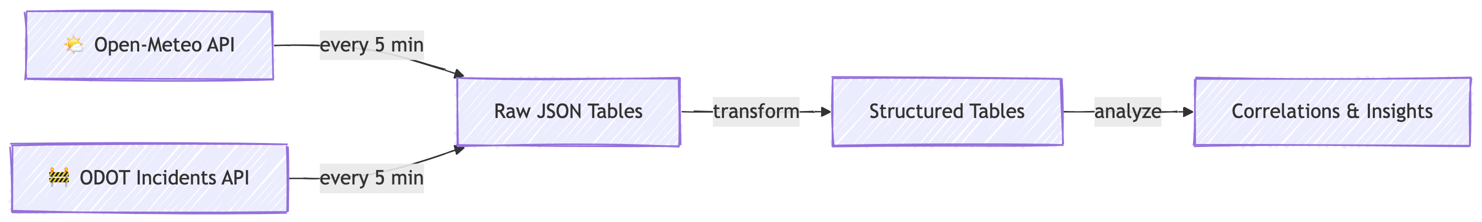
A Real-Time Data Pipeline

We are building a pipeline that continuously collects data from two public APIs, stores it in a cloud database, and transforms it into structured tables ready for analysis.

Every 5 minutes, our pipeline wakes up, fetches fresh data, and stores it. No human intervention required. You could go on vacation and come back to weeks of data. (Please do not go on vacation mid-semester.) 🏖️

The ELT Pattern

This pipeline follows the ELT pattern:

Extract — pull raw data from web APIs
Load — store the raw JSON directly into PostgreSQL
Transform — convert raw JSON into structured, queryable tables

This is different from traditional ETL (Extract, Transform, Load), where you clean the data before storing it. With ELT, we store first and ask questions later. The database is powerful enough to handle the transformation. 💪

Why ELT Over ETL?

Raw data is preserved — if your transformation has a bug, you still have the originals
Schema flexibility — JSON can hold anything; you decide the structure later
PostgreSQL is great at this — JSONB operators make transformation fast and expressive
Decoupled stages — ingestion and transformation run independently

The Use Case

🌧️ Does Weather Cause Traffic Incidents?

Here is our research question:

Do weather conditions correlate with traffic incidents on Oregon highways?

We will collect:

Weather data for Portland, OR (temperature, humidity, precipitation, wind, weather codes) from Open-Meteo
Traffic incident data for all of Oregon (crashes, closures, hazards, construction) from ODOT TripCheck via ArcGIS

With continuous 5-minute polling, we can explore:

Correlations — do more incidents happen during rain or high wind?
Lag correlations — does a weather event precede a spike in incidents by 30-60 minutes?
Time bucketing — what does the hourly or daily pattern look like?

This is real data engineering: collect, store, transform, analyze. Let’s build it. 🔧

Phase 1: Cloud Infrastructure

What is Railway?

Your Cloud Platform

Railway is a Platform-as-a-Service (PaaS) that makes deploying databases, Docker containers, and web services ridiculously easy.

Think of it as the friendly neighborhood version of AWS or Azure:

Feature	AWS / Azure	Railway
Setup time	Hours to days	Minutes
Learning curve	Steep (IAM, VPCs, security groups…)	Gentle
Pricing	Complex (pay per everything)	Simple ($5/month hobby tier)
Target audience	Enterprise teams	Developers, students, small projects
Docker support	✅ (ECS, EKS, ACI…)	✅ (just paste an image name)
Managed Postgres	✅ (RDS, Azure DB)	✅ (one click)

How We Will Use Railway

In this lab, Railway will host:

A PostgreSQL database — our central data store
Two Docker containers — one for each API, running on cron schedules

Railway handles networking, environment variables, scheduling, and deployment. We just configure and go.

Creating Your Railway Account

Step 2: Upgrade to the Hobby Plan

Railway’s free tier is very limited. The Hobby plan costs $5/month and gives you enough resources for this project.

Go to your Railway dashboard
Click your profile icon (bottom left) → “Account Settings”
Under “Plan”, select “Hobby”
Enter a credit card — you get a $5 credit each month
Our usage will stay well within that $5

Yes, you need a credit card. No, you will not get a surprise bill. Railway caps hobby usage at $5 unless you explicitly upgrade. 💳

Step 3: Create a New Project

From your Railway dashboard, click “New Project”
Select “Empty Project”
Railway creates a project with a default environment

Step 4: Rename Your Environment

The default environment name is not very descriptive. Let’s fix that.

In your project, look at the top bar where it says the environment name
Right-click or click the dropdown next to the environment name
Choose “Rename”
Name it something meaningful: Traffic-Weather-Pipeline

Good naming is not optional. When you have five projects and twelve environments, “production” means nothing. “Traffic-Weather-Pipeline” tells you exactly what is running. 🏷️

Phase 2: Database Setup

Provisioning PostgreSQL

Step 1: Add a Postgres Service

In your Traffic-Weather-Pipeline project, click “New”
Select “Database”
Choose “PostgreSQL”
Railway provisions the database automatically — this takes about 30 seconds

You now have a fully managed PostgreSQL instance running in the cloud. No installation, no configuration files, no pg_hba.conf nightmares. 🎉

Step 2: Get Your Connection URL

Click on the Postgres service in your project
Open the “Variables” tab
Find and copy the DATABASE_PUBLIC_URL

It looks something like:

postgresql://postgres:AbCdEf123@roundhouse.proxy.rlwy.net:20848/railway

This URL contains everything needed to connect: username, password, host, port, and database name. Guard it like a secret — anyone with this URL has full access to your database. 🔐

Step 3: Connect with Beekeeper Studio

Beekeeper Studio is great to use with Railway because you can import a database connection URL directly. pgAdmin works too, but we have to set up the connection manually.

IMPORTANT: make sure you note which database you’re connected to when switching between tasks. Often people find (or don’t find) what they are expecting to see and worry their databases are gone. You’re probably just connected to the wrong database server.

Open Beekeeper Studio
Click “New Connection”
Choose PostgreSQL
Click “Import from URL” and paste your DATABASE_PUBLIC_URL
Click “Connect”

You should see an empty database. Perfect. We are about to fill it.

Creating Raw Storage Tables

The Staging Tables

Before we can ingest data, we need tables to receive it. These are append-only staging tables — every API response gets stored as a raw JSON blob with a timestamp.

CREATE TABLE weather_json (
    id SERIAL PRIMARY KEY,
    raw_json JSONB NOT NULL,
    created_at TIMESTAMPTZ NOT NULL DEFAULT NOW()
);

CREATE TABLE incidents_json (
    id SERIAL PRIMARY KEY,
    raw_json JSONB NOT NULL,
    created_at TIMESTAMPTZ NOT NULL DEFAULT NOW()
);

Run this SQL in Beekeeper Studio.

Why JSONB?

PostgreSQL has two JSON types: JSON and JSONB.

JSON stores the raw text exactly as received
JSONB stores it in a decomposed binary format

We use JSONB because:

It is faster to query — PostgreSQL can index and search inside it
It supports operators like ->, ->>, @>, and ?
It removes duplicate keys and does not preserve whitespace (we don’t care about formatting)
It is the right choice for any serious JSON work in Postgres

Why Store Raw JSON at All?

Great question. Three reasons:

Data preservation — if your transformation logic has a bug, the raw data is still there
Schema evolution — APIs change; raw JSON captures whatever they send
Debugging — when something looks wrong downstream, you can inspect the exact payload

This is the “L” in ELT. Load first, transform later.

Phase 3: Understanding the APIs

What is an API?

Application Programming Interface

An API is a structured way for programs to talk to each other. When you visit a website, your browser renders HTML for humans. When you call an API, you get structured data for programs.

The APIs we are using are REST APIs — they use standard HTTP requests (like typing a URL in your browser) and return data in JSON format.

You send a request (a URL with parameters)
The server processes it
You get back structured data (JSON)

No API keys required for either of our data sources. They are free and public. 🎁

What is JSON?

JavaScript Object Notation

JSON (JavaScript Object Notation) is the most common format for data exchange on the web. If APIs are the highways of the internet, JSON is the cargo.

JSON has a few simple building blocks:

Objects — key-value pairs wrapped in curly braces {}
Arrays — ordered lists wrapped in square brackets []
Values — strings, numbers, booleans, null, objects, or arrays

{
  "name": "Portland",
  "temperature": 51.6,
  "raining": true,
  "alerts": ["wind advisory", "flood watch"],
  "location": {
    "latitude": 45.52,
    "longitude": -122.68
  }
}

Everything is text. Everything is human-readable. Everything nests. That is the beauty (and sometimes the pain) of JSON. 📦

API #1: Open-Meteo Weather

The URL

https://api.open-meteo.com/v1/forecast?latitude=45.52&longitude=-122.68&timezone=America%2FLos_Angeles&current=temperature_2m,relative_humidity_2m,precipitation,weather_code,wind_speed_10m,wind_direction_10m&temperature_unit=fahrenheit&wind_speed_unit=mph&precipitation_unit=inch

Query Parameters Explained

https://api.open-meteo.com/v1/forecast?latitude=45.52&longitude=-122.68&timezone=America%2FLos_Angeles&current=temperature_2m,relative_humidity_2m,precipitation,weather_code,wind_speed_10m,wind_direction_10m&temperature_unit=fahrenheit&wind_speed_unit=mph&precipitation_unit=inch

Parameter	Value	What It Does
`latitude`	`45.52`	Latitude for downtown Portland, OR
`longitude`	`-122.68`	Longitude for downtown Portland, OR
`current`	`temperature_2m,...`	Which current-conditions fields to return
`temperature_unit`	`fahrenheit`	Because this is America 🇺🇸
`wind_speed_unit`	`mph`	Miles per hour
`precipitation_unit`	`inch`	Inches of precipitation

The current parameter is a comma-separated list of weather variables. We are requesting:

temperature_2m — air temperature at 2 meters above ground
relative_humidity_2m — humidity percentage
precipitation — current precipitation amount
weather_code — WMO weather condition code (0 = clear, 61 = rain, 71 = snow, etc.)
wind_speed_10m — wind speed at 10 meters above ground
wind_direction_10m — wind direction in degrees (0° = north, 90° = east, etc.)

Sample JSON Response

{
  "latitude": 45.528744,
  "longitude": -122.696236,
  "generationtime_ms": 0.13,
  "utc_offset_seconds": 0,
  "timezone": "GMT",
  "timezone_abbreviation": "GMT",
  "elevation": 31,
  "current_units": {
    "time": "iso8601",
    "interval": "seconds",
    "temperature_2m": "°F",
    "relative_humidity_2m": "%",
    "precipitation": "inch",
    "weather_code": "wmo code",
    "wind_speed_10m": "mp/h",
    "wind_direction_10m": "°"
  },
  "current": {
    "time": "2026-03-04T22:30",
    "interval": 900,
    "temperature_2m": 51.6,
    "relative_humidity_2m": 73,
    "precipitation": 0.114,
    "weather_code": 73,
    "wind_speed_10m": 10.5,
    "wind_direction_10m": 268
  }
}

Reading the Response

The important stuff lives inside the "current" object:

Key	Example Value	Meaning
`time`	`"2026-03-04T22:30"`	When this reading was taken (UTC)
`interval`	`900`	Update interval in seconds (15 min)
`temperature_2m`	`51.6`	Temperature in °F
`relative_humidity_2m`	`73`	Humidity as a percentage
`precipitation`	`0.114`	Current precipitation in inches
`weather_code`	`73`	WMO code (73 = moderate snow fall)
`wind_speed_10m`	`10.5`	Wind speed in mph
`wind_direction_10m`	`268`	Wind from the west (270° = due west)

The current_units object tells you the unit for each field — useful for documentation and sanity-checking.

API #2: ODOT Traffic Incidents (ArcGIS)

The URL

https://services.arcgis.com/uUvqNMGPm7axC2dD/ArcGIS/rest/
  services/TripCheck_Incidents_Data_Upload_view/
  FeatureServer/0/query
  ?where=1%3D1
  &outFields=*
  &f=json
  &resultRecordCount=500

This is an ArcGIS Feature Service — a standard way to serve geospatial data. ODOT (Oregon Department of Transportation) publishes live traffic incident data through this service, which powers TripCheck.com.

Query Parameters Explained

Parameter	Value	What It Does
`where`	`1=1`	SQL-style filter — `1=1` means “give me everything”
`outFields`	`*`	Return all available fields (not just a subset)
`f`	`json`	Return format — we want JSON
`resultRecordCount`	`500`	Maximum number of records to return per request

The where=1%3D1 might look weird — that %3D is just the URL-encoded version of =. So it is where=1=1, which in SQL means “all rows.” ArcGIS borrowed SQL syntax for its query interface. 🤓

Sample JSON Response

The response wraps each incident in a features array. Each feature has attributes and geometry:

{
  "objectIdFieldName": "ObjectId",
  "features": [
    {
      "attributes": {
        "attributes_incidentId": 776079,
        "attributes_route": "OR-229",
        "attributes_locationName": "SILETZ",
        "attributes_odotCategoryDescript": "Crash or Hazard",
        "attributes_odotSeverityDescript": "Closure",
        "attributes_eventTypeName": "Obstruction",
        "attributes_eventSubTypeName": "Landslide",
        "attributes_comments": "A landslide has occurred. Use an alternate route.",
        "attributes_incidentDirection": "",
        "attributes_startLatitude": 44.80854,
        "attributes_startLongitude": -123.96581,
        "attributes_endLatitude": 44.80135,
        "attributes_endLongitude": -123.95331,
        "attributes_beginMP": 14,
        "attributes_endMP": 15,
        "attributes_lastUpdated": 1766095973878,
        "attributes_startTime": null,
        "attributes_odotSeverityID": 4,
        "attributes_iconType": 29,
        "ObjectId": 3095775,
        "GlobalID": "402bad59-3882-4088-93cc-8fd17b9657ac"
      },
      "geometry": {
        "x": -13799810.84,
        "y": 5591430.22
      }
    }
  ]
}

Key Fields We Care About

Field	Example	Meaning
`attributes_incidentId`	`776079`	Unique incident identifier
`attributes_route`	`"OR-229"`	Highway or route name
`attributes_locationName`	`"SILETZ"`	Nearest town or landmark
`attributes_odotCategoryDescript`	`"Crash or Hazard"`	Incident category
`attributes_odotSeverityDescript`	`"Closure"`	How bad it is
`attributes_eventTypeName`	`"Obstruction"`	General event type
`attributes_eventSubTypeName`	`"Landslide"`	Specific event subtype
`attributes_comments`	`"A landslide has..."`	Human-readable description
`attributes_startLatitude`	`44.80854`	Where it starts (lat)
`attributes_startLongitude`	`-123.96581`	Where it starts (lon)
`attributes_lastUpdated`	`1766095973878`	Unix timestamp in milliseconds

The geometry field uses Web Mercator projection (EPSG:3857) — those giant numbers are projected coordinates, not lat/lon. The actual lat/lon is in the attributes. GIS is fun. 🗺️

Phase 4: Deploying the Ingestion Services

Using the api2db Template

What is api2db?

api2db is a Docker container that does one thing well:

Fetches data from a URL
Stores the raw JSON response in a PostgreSQL table

It runs once per execution and is designed to be triggered on a cron schedule. No code to write — you configure it entirely through environment variables.

Deploying with the Railway Template

I have created a Railway template that makes deployment a one-click process. 🚀

Open this link: railway.com/deploy/api2db-template
Click “Configure”
Choose your environment — select Traffic-Weather-Pipeline (the one you renamed earlier)
Fill in the environment variables (next slides)
Click “Deploy”

You will deploy this template twice — once for weather, once for traffic incidents.

What is Cron?

Scheduled Task Execution

Cron is a time-based job scheduler. It uses a simple expression format to define when something should run.

The format is five fields:

┌───────────── minute (0-59)
│ ┌───────────── hour (0-23)
│ │ ┌───────────── day of month (1-31)
│ │ │ ┌───────────── month (1-12)
│ │ │ │ ┌───────────── day of week (0-6, Sun=0)
│ │ │ │ │
* * * * *

Some examples:

Expression	Meaning
`/5 * * *`	Every 5 minutes
`0 * * * *`	Every hour, on the hour
`0 9 * * 1`	Every Monday at 9:00 AM
`0 0 * * *`	Midnight every day

*/5 means “every value divisible by 5” — so minutes 0, 5, 10, 15, 20, 25, 30, 35, 40, 45, 50, 55.

Bookmark crontab.guru — it translates cron expressions into plain English. It will save your life. 🔖

Deploying the Weather Ingestion Service

Step 1: Deploy the Template

Open railway.com/deploy/api2db-template
Click “Configure”
Select your Traffic-Weather-Pipeline environment

Step 2: Set Environment Variables

When the template asks for configuration, enter:

Variable	Value
`SITE_URL`	`https://api.open-meteo.com/v1/forecast?latitude=45.52&longitude=-122.68&current=temperature_2m,relative_humidity_2m,precipitation,weather_code,wind_speed_10m,wind_direction_10m&temperature_unit=fahrenheit&wind_speed_unit=mph&precipitation_unit=inch`
`TABLE_NAME`	`weather_json`

The template will automatically connect DATABASE_URL to your Postgres service using Railway’s internal variable referencing.

Step 3: Set the Cron Schedule

After deployment, click into the new service
Go to the “Settings” tab
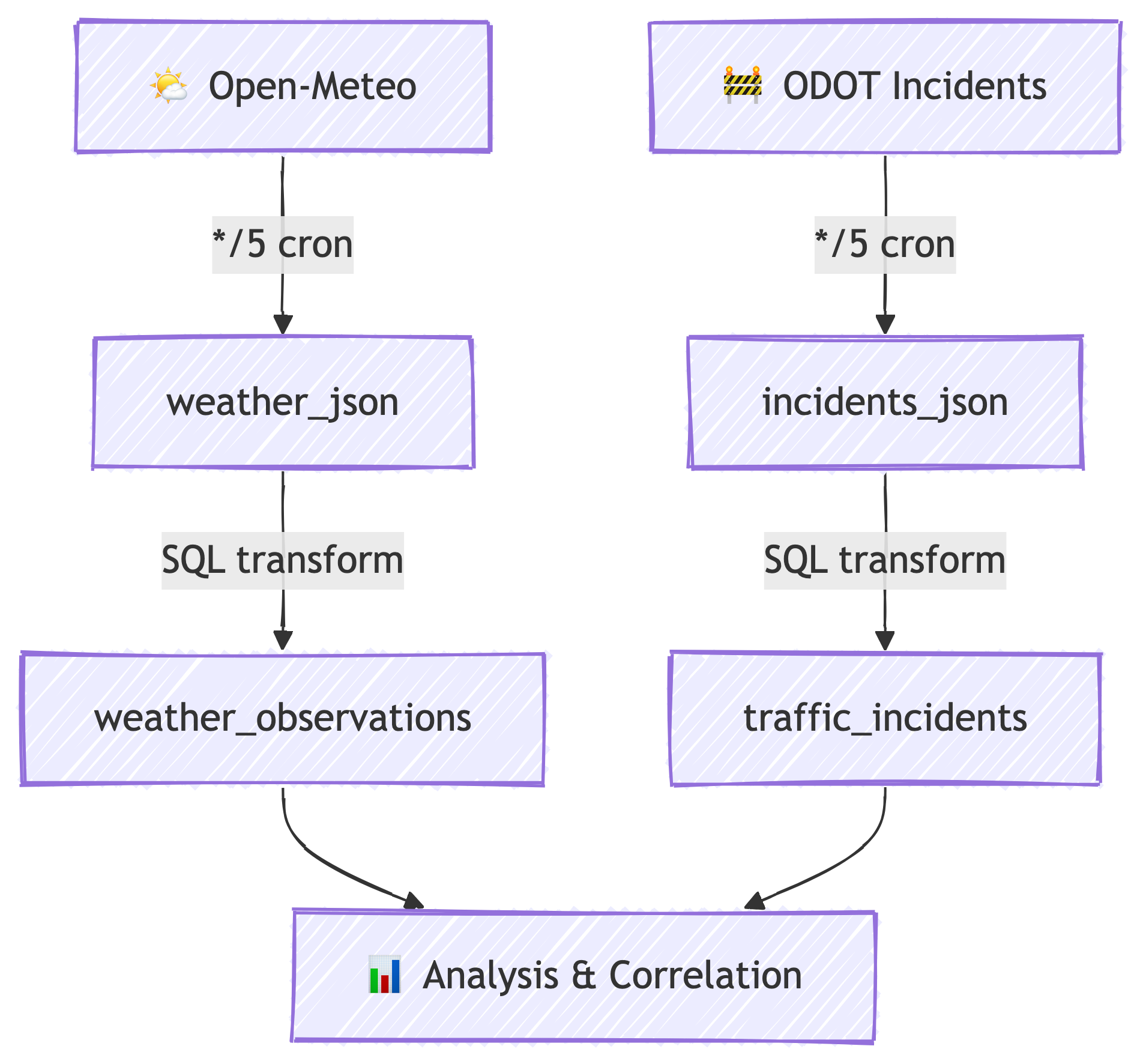
Under “Cron Schedule”, enter: */5 * * * *
Click “Deploy”

This service will now wake up every 5 minutes, fetch the weather data, store it in weather_json, and go back to sleep. 💤

Step 4: Rename the Service

The template gives it a generic name. Rename it to something useful:

In the service Settings, find the service name
Rename it to weather-ingestion

Deploying the Incidents Ingestion Service

Step 1: Deploy the Template Again

Open railway.com/deploy/api2db-template again
Click “Configure”
Select your Traffic-Weather-Pipeline environment (same one!)

Step 2: Set Environment Variables

Variable	Value
`SITE_URL`	`https://services.arcgis.com/uUvqNMGPm7axC2dD/ArcGIS/rest/services/TripCheck_Incidents_Data_Upload_view/FeatureServer/0/query?where=1%3D1&outFields=*&f=json&resultRecordCount=500`
`TABLE_NAME`	`incidents_json`

Step 3: Set the Cron Schedule

Same as before:

Settings → Cron Schedule → */5 * * * *
Deploy

Step 4: Rename the Service

Rename to incidents-ingestion.

Verifying the Data

Check That It is Working

After waiting ~5 minutes for the first cron trigger, run these queries in Beekeeper Studio:

SELECT COUNT(*) FROM weather_json;
SELECT COUNT(*) FROM incidents_json;

If both return at least 1 row, you are in business. ✅

Inspect the actual data:

SELECT id, created_at,
       raw_json->'current'->>'temperature_2m' AS temp_f
FROM weather_json
ORDER BY created_at DESC
LIMIT 5;

SELECT id, created_at,
       jsonb_array_length(raw_json->'features') AS incident_count
FROM incidents_json
ORDER BY created_at DESC
LIMIT 5;

If you see timestamps and data, congratulations — you have two live data streams flowing into your database. You are officially a data engineer. Put it on your resume. 🎉

Troubleshooting:

Check the “Deployments” tab — did the cron job run?
Check the “Logs” tab — any error messages?
Double-check SITE_URL for typos (especially that long ArcGIS URL)
Make sure you selected the right environment when deploying

Phase 5: Data Transformation

From Raw to Structured

Why Transform?

Raw JSON is great for storage but terrible for analysis. Try writing a query to find the average temperature grouped by hour from a pile of nested JSON objects. It is not fun. 😤

Transformation takes our raw JSON and extracts the fields we care about into proper columns with proper types. After transformation:

Temperatures are DOUBLE PRECISION, not strings buried in JSON
Timestamps are TIMESTAMPTZ, not nested inside objects
You can GROUP BY, JOIN, and aggregate like a normal person

This is the “T” in ELT.

PostgreSQL JSON Operators

Your Transformation Toolkit

PostgreSQL provides powerful operators for working with JSONB:

Operator	Returns	Example	Result
`->`	JSON element	`raw_json->'current'`	`{"time":"...","temperature_2m":51.6}`
`->>`	Text	`raw_json->'current'->>'temperature_2m'`	`'51.6'` (as text)
`#>`	JSON at path	`raw_json #> '{current,time}'`	`"2026-03-04T22:30"`
`#>>`	Text at path	`raw_json #>> '{current,time}'`	`2026-03-04T22:30`

The key difference:

-> navigates into JSON and returns JSON (for further chaining)
->> navigates into JSON and returns text (for casting to other types)

You will almost always use -> to dig into nested objects and then ->> at the final level to extract a text value, which you then cast to the appropriate type.

Chaining Operators

To get the temperature from our weather JSON:

-- Step by step:
raw_json -> 'current'                    -- gets the "current" object (as JSON)
raw_json -> 'current' ->> 'temperature_2m'  -- gets "51.6" (as text)
(raw_json -> 'current' ->> 'temperature_2m')::DOUBLE PRECISION  -- gets 51.6 (as a number)

The :: is PostgreSQL’s cast operator. It converts text to whatever type you need.

Expanding Arrays with jsonb_array_elements

The incidents API returns an array of features. To work with individual incidents, we need to unnest that array:

SELECT jsonb_array_elements(raw_json -> 'features') AS feature
FROM incidents_json;

jsonb_array_elements() takes a JSON array and returns one row per element. If the array has 200 incidents, you get 200 rows. This is how we go from “one big blob” to “one row per incident.”

Designing the Target Tables

Weather Observations Table

CREATE TABLE weather_observations (
    id SERIAL PRIMARY KEY,
    observed_at TIMESTAMPTZ NOT NULL,
    temperature_f DOUBLE PRECISION,
    humidity_pct DOUBLE PRECISION,
    precipitation_in DOUBLE PRECISION,
    weather_code SMALLINT,
    wind_speed_mph DOUBLE PRECISION,
    wind_direction_deg DOUBLE PRECISION,
    ingested_at TIMESTAMPTZ NOT NULL
);

Traffic Incidents Table

CREATE TABLE traffic_incidents (
    id SERIAL PRIMARY KEY,
    incident_id INTEGER NOT NULL,
    route TEXT,
    location_name TEXT,
    category TEXT,
    severity TEXT,
    event_type TEXT,
    event_subtype TEXT,
    comments TEXT,
    direction TEXT,
    start_lat DOUBLE PRECISION,
    start_lon DOUBLE PRECISION,
    end_lat DOUBLE PRECISION,
    end_lon DOUBLE PRECISION,
    begin_milepost DOUBLE PRECISION,
    end_milepost DOUBLE PRECISION,
    last_updated TIMESTAMPTZ,
    ingested_at TIMESTAMPTZ NOT NULL
);

Run both of these in Beekeeper Studio.

Notice how each table has an ingested_at column — this records when we captured this data, which is different from when the event occurred. That distinction matters for time-series analysis.

Writing the Transformation Queries

Weather Transformation

BEGIN;

INSERT INTO weather_observations (
    observed_at,
    temperature_f,
    humidity_pct,
    precipitation_in,
    weather_code,
    wind_speed_mph,
    wind_direction_deg,
    ingested_at
)
SELECT
    (raw_json #>> '{current,time}')::TIMESTAMPTZ
        AS observed_at,
    (raw_json #>> '{current,temperature_2m}')::DOUBLE PRECISION
        AS temperature_f,
    (raw_json #>> '{current,relative_humidity_2m}')::DOUBLE PRECISION
        AS humidity_pct,
    (raw_json #>> '{current,precipitation}')::DOUBLE PRECISION
        AS precipitation_in,
    (raw_json #>> '{current,weather_code}')::SMALLINT
        AS weather_code,
    (raw_json #>> '{current,wind_speed_10m}')::DOUBLE PRECISION
        AS wind_speed_mph,
    (raw_json #>> '{current,wind_direction_10m}')::DOUBLE PRECISION
        AS wind_direction_deg,
    created_at AS ingested_at
FROM weather_json;

DELETE FROM weather_json;

COMMIT;

What is Happening Here?

Let’s break it down:

BEGIN — start a transaction (all-or-nothing)
INSERT INTO ... SELECT — extract fields from JSON and insert into the structured table
#>> — path-based JSON extraction returning text
::DOUBLE PRECISION — cast the text to a number
DELETE FROM weather_json — clear the raw data (it has been processed)
COMMIT — finalize the transaction

If the INSERT fails, the DELETE never happens. Your raw data stays safe. That is why we use transactions. This is how adults write SQL. 💪

Incidents Transformation

BEGIN;

WITH features AS (
    SELECT
        created_at,
        jsonb_array_elements(raw_json -> 'features') AS feature
    FROM incidents_json
)
INSERT INTO traffic_incidents (
    incident_id,
    route,
    location_name,
    category,
    severity,
    event_type,
    event_subtype,
    comments,
    direction,
    start_lat,
    start_lon,
    end_lat,
    end_lon,
    begin_milepost,
    end_milepost,
    last_updated,
    ingested_at
)
SELECT
    (feature -> 'attributes' ->> 'attributes_incidentId')::INTEGER,
    feature -> 'attributes' ->> 'attributes_route',
    feature -> 'attributes' ->> 'attributes_locationName',
    feature -> 'attributes' ->> 'attributes_odotCategoryDescript',
    feature -> 'attributes' ->> 'attributes_odotSeverityDescript',
    feature -> 'attributes' ->> 'attributes_eventTypeName',
    feature -> 'attributes' ->> 'attributes_eventSubTypeName',
    feature -> 'attributes' ->> 'attributes_comments',
    feature -> 'attributes' ->> 'attributes_incidentDirection',
    (feature -> 'attributes' ->> 'attributes_startLatitude')::DOUBLE PRECISION,
    (feature -> 'attributes' ->> 'attributes_startLongitude')::DOUBLE PRECISION,
    (feature -> 'attributes' ->> 'attributes_endLatitude')::DOUBLE PRECISION,
    (feature -> 'attributes' ->> 'attributes_endLongitude')::DOUBLE PRECISION,
    (feature -> 'attributes' ->> 'attributes_beginMP')::DOUBLE PRECISION,
    (feature -> 'attributes' ->> 'attributes_endMP')::DOUBLE PRECISION,
    TO_TIMESTAMP(
        (feature -> 'attributes' ->> 'attributes_lastUpdated')::BIGINT / 1000.0
    ),
    created_at
FROM features;

DELETE FROM incidents_json;

COMMIT;

What is a CTE?

That WITH features AS (...) is a Common Table Expression (CTE).

A CTE is a temporary named result set that exists for the duration of a single query. Think of it as scratch paper for your SQL — you break a complex problem into named steps.

WITH step1 AS (
    -- first calculation
),
step2 AS (
    -- uses step1
)
SELECT * FROM step2;

In our case, the CTE unnests the JSON array first, giving us one row per incident. Then the outer query extracts the fields from each incident. Without the CTE, we would need a messy subquery. CTEs keep things readable. 📝

The Timestamp Trick

Notice this line in the incidents transformation:

TO_TIMESTAMP(
    (feature -> 'attributes' ->> 'attributes_lastUpdated')::BIGINT / 1000.0
)

The ODOT API returns timestamps as Unix milliseconds (e.g., 1766095973878). PostgreSQL’s TO_TIMESTAMP() expects seconds. So we divide by 1000 to convert.

1766095973878 / 1000.0 = 1766095973.878 → 2025-12-18 17:52:53.878

Always check your timestamp formats. APIs are not consistent about this. Some use seconds, some milliseconds, some ISO strings. Welcome to data engineering. 🕐

Verifying the Transformation

Check the Results

After running both transformation queries:

SELECT COUNT(*) FROM weather_observations;
SELECT * FROM weather_observations
ORDER BY ingested_at DESC LIMIT 5;

SELECT COUNT(*) FROM traffic_incidents;
SELECT * FROM traffic_incidents
ORDER BY last_updated DESC LIMIT 10;

-- The raw tables should be empty now
SELECT COUNT(*) FROM weather_json;    -- should be 0
SELECT COUNT(*) FROM incidents_json;  -- should be 0

If you see structured rows in the target tables and empty raw tables, the transformation worked. Raw JSON in, clean columns out. Beautiful. ✨

Phase 6: Analysis Preview

What Can We Do Now?

Sample Analytical Queries

With structured data, the real fun begins. Here are some queries to try once you have accumulated some data:

Incident counts by category:

SELECT category, COUNT(*) AS total
FROM traffic_incidents
GROUP BY category
ORDER BY total DESC;

Average temperature when incidents were reported:

SELECT
    ROUND(AVG(w.temperature_f)::NUMERIC, 1) AS avg_temp,
    ROUND(AVG(w.wind_speed_mph)::NUMERIC, 1) AS avg_wind,
    COUNT(DISTINCT t.incident_id) AS incident_count
FROM traffic_incidents t
JOIN weather_observations w
    ON DATE_TRUNC('hour', t.last_updated)
     = DATE_TRUNC('hour', w.observed_at);

Hourly incident counts (time bucketing):

SELECT
    DATE_TRUNC('hour', last_updated) AS hour,
    COUNT(*) AS incidents
FROM traffic_incidents
GROUP BY hour
ORDER BY hour;

These are just starting points. With enough data, you could build lag correlation analyses, weather severity scoring, and time-series visualizations. The pipeline keeps running — your dataset grows every 5 minutes. 📈

Recap

What We Built

Six Phases, One Pipeline

Phase	What We Did
1. Cloud Infrastructure	Set up Railway account, project, and environment
2. Database Setup	Provisioned PostgreSQL, created raw JSON tables
3. Understanding APIs	Explored Open-Meteo and ODOT endpoints and their JSON
4. Ingestion	Deployed two api2db containers on 5-minute cron schedules
5. Transformation	Wrote SQL to extract JSON into structured tables
6. Analysis	Queried structured data for insights

Key Concepts

ELT pattern — extract, load raw, transform later
JSONB — PostgreSQL’s binary JSON type for flexible storage and powerful querying
JSON operators (->, ->>, #>>) — navigate and extract from nested JSON
jsonb_array_elements() — unnest JSON arrays into rows
Cron scheduling — time-based automation for periodic data collection
Transactions — atomic operations to keep data consistent
CTEs — readable, step-by-step query composition

References

Railway Documentation. https://docs.railway.app
PostgreSQL JSON Functions. https://www.postgresql.org/docs/current/functions-json.html
Open-Meteo API Documentation. https://open-meteo.com/en/docs
ODOT TripCheck. https://tripcheck.com
ArcGIS REST API. https://developers.arcgis.com/rest/
Crontab Guru. https://crontab.guru/
Beekeeper Studio. https://www.beekeeperstudio.io/
WMO Weather Codes. https://www.nodc.noaa.gov/archive/arc0021/0002199/1.1/data/0-data/HTML/WMO-CODE/WMO4677.HTM

Lecture 08-2: Web Data Pipelines

The Big Picture

What Are We Building?

A Real-Time Data Pipeline

The ELT Pattern

Why ELT Over ETL?

The Use Case

🌧️ Does Weather Cause Traffic Incidents?

Phase 1: Cloud Infrastructure

What is Railway?

Your Cloud Platform

How We Will Use Railway

Creating Your Railway Account

Step 1: Sign Up with GitHub

Step 2: Upgrade to the Hobby Plan

Step 3: Create a New Project

Step 4: Rename Your Environment

Phase 2: Database Setup

Provisioning PostgreSQL

Step 1: Add a Postgres Service

Step 2: Get Your Connection URL

Step 3: Connect with Beekeeper Studio

Creating Raw Storage Tables

The Staging Tables

Why JSONB?

Why Store Raw JSON at All?

Phase 3: Understanding the APIs

What is an API?

Application Programming Interface

What is JSON?

JavaScript Object Notation

API #1: Open-Meteo Weather

The URL

Query Parameters Explained

Sample JSON Response

Reading the Response

API #2: ODOT Traffic Incidents (ArcGIS)

The URL

Query Parameters Explained

Sample JSON Response

Key Fields We Care About

Phase 4: Deploying the Ingestion Services

Using the api2db Template

What is api2db?

Deploying with the Railway Template

What is Cron?

Scheduled Task Execution

Deploying the Weather Ingestion Service

Step 1: Deploy the Template

Step 2: Set Environment Variables

Step 3: Set the Cron Schedule

Step 4: Rename the Service

Deploying the Incidents Ingestion Service

Step 1: Deploy the Template Again

Step 2: Set Environment Variables

Step 3: Set the Cron Schedule

Step 4: Rename the Service

Verifying the Data

Check That It is Working

Phase 5: Data Transformation

From Raw to Structured

Why Transform?

PostgreSQL JSON Operators

Your Transformation Toolkit

Chaining Operators

Expanding Arrays with jsonb_array_elements

Designing the Target Tables

Weather Observations Table

Traffic Incidents Table

Writing the Transformation Queries

Weather Transformation

What is Happening Here?

Incidents Transformation

What is a CTE?

The Timestamp Trick

Verifying the Transformation

Check the Results

Phase 6: Analysis Preview

What Can We Do Now?

Sample Analytical Queries