Lecture 09-1: Advanced Statistics with Flight and Weather Data
DATA 503: Fundamentals of Data Engineering
March 11, 2026
Part 1: The Data Pipeline So Far
For two weeks, your Railway scrapers have been quietly hoarding JSON like digital squirrels.
Time to crack open the acorns.
Our Data Collection Architecture
What We Built
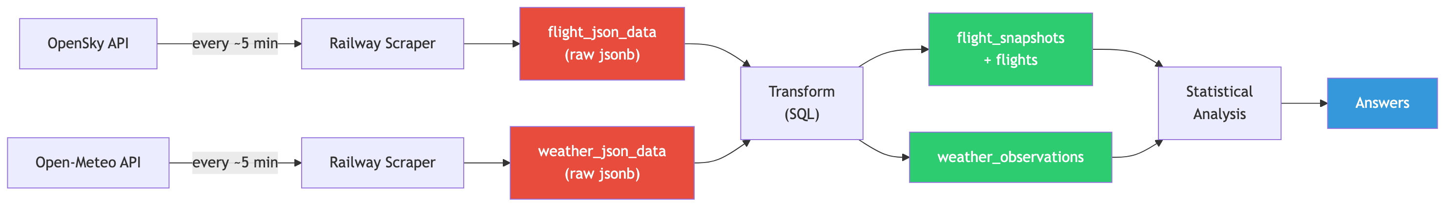
Over the past two weeks, you deployed two API scrapers on Railway:
| Scraper | Source | Frequency | Rows Collected |
|---|---|---|---|
| Flight tracker | OpenSky Network API | ~5 min | ~2,130 snapshots |
| Weather monitor | Open-Meteo API | ~5 min | ~1,877 observations |
Both scrapers dump raw JSON into Railway Postgres. No parsing, no cleaning, no opinions. Just raw data.
This is the staging layer of our pipeline, and today we promote that data to something useful.
The Pipeline: From JSON to Insight
Red = messy staging. Green = clean, normalized. Blue = the whole reason we did this.
The Staging Tables
Both staging tables have the same dead-simple structure:
One column for the ID, one for the entire JSON blob, one for when we grabbed it.
This is the database equivalent of throwing everything in a cardboard box during a move. It works, but you would not want to live like that.
Part 2: Understanding Our JSON Data
Before we can transform the data, we need to understand what we are actually looking at.
Time to open the cardboard boxes.
Exploring JSON in PostgreSQL
PostgreSQL JSON Operators: Your Swiss Army Knife
| Operator | Returns | Example |
|---|---|---|
-> |
JSON object/array | raw_json->'states' returns a JSON array |
->> |
Text | raw_json->>'time' returns '1772503243' as text |
->N |
Nth array element (JSON) | state->0 returns first element as JSON |
->>N |
Nth array element (text) | state->>1 returns callsign as text |
jsonb_array_elements() |
Set of JSON values | Unnests an array into rows |
The difference between -> and ->> is critical: one gives you JSON, the other gives you text. Mix them up and your casts will fail in confusing ways.
Flight JSON Structure
Each row in flight_json_data contains a snapshot from the OpenSky Network API:
{
  "time": 1772503243,
  "states": [
    [
      "a88bb8",        -- [0] icao24 transponder address
      "N65PT   ",      -- [1] callsign (8 chars, trailing spaces)
      "United States", -- [2] origin_country
      1772503243,      -- [3] time_position
      1772503243,      -- [4] last_contact
      -122.23,         -- [5] longitude
      45.5592,         -- [6] latitude
      731.52,          -- [7] baro_altitude (meters, nullable)
      false,           -- [8] on_ground
      66.19,           -- [9] velocity (m/s)
      78.34,           -- [10] true_track (degrees)
      0.65,            -- [11] vertical_rate (m/s, nullable)
      null,            -- [12] sensors (usually null)
      754.38,          -- [13] geo_altitude (meters, nullable)
      null,            -- [14] squawk (nullable)
      false,           -- [15] spi
      0                -- [16] position_source
    ]
  ]
}
Notice: states is an array of arrays. Each inner array is one aircraft. And sometimes states is just null because apparently nobody was flying over Portland at 3 AM. Shocking.
Exploring Flight Data
Let’s peek at what we have:
-- How many snapshots?
SELECT count(*) FROM flight_json_data;

-- Look at one snapshot's timestamp
SELECT raw_json->>'time' AS api_time,
       created_at AS collected_at
FROM flight_json_data
LIMIT 1;

-- How many aircraft in each snapshot?
SELECT id,
       jsonb_array_length(raw_json->'states') AS num_aircraft
FROM flight_json_data
WHERE raw_json->'states' IS NOT NULL
    AND raw_json->>'states' != 'null'
ORDER BY num_aircraft DESC
LIMIT 10;
That WHERE clause filters out snapshots where nobody was flying. Without it, jsonb_array_length will throw errors on null values, and your query will be reduced to atoms.
Unnesting Flight Arrays
The real magic is jsonb_array_elements(), which turns one row with an array of 30 aircraft into 30 rows with one aircraft each:
SELECT
    raw_json->>'time' AS snapshot_time,
    state->>0 AS icao24,
    TRIM(state->>1) AS callsign,
    state->>2 AS origin_country,
    (state->>5)::numeric AS longitude,
    (state->>6)::numeric AS latitude,
    (state->>7)::numeric AS baro_altitude,
    (state->>8)::boolean AS on_ground,
    (state->>9)::numeric AS velocity
FROM flight_json_data,
     jsonb_array_elements(raw_json->'states') AS state
WHERE raw_json->'states' IS NOT NULL
    AND raw_json->>'states' != 'null'
LIMIT 20;
Notice the TRIM() on callsign. OpenSky pads callsigns to 8 characters with trailing spaces, because apparently fixed-width strings never really died.
Weather JSON Structure
Weather data is simpler. Each row is one observation, no arrays to unnest:
Three numbers we care about: temperature, wind speed, and weather code.
Exploring Weather Data
-- Peek at weather observations
SELECT
    raw_json->'current'->>'time' AS obs_time,
    (raw_json->'current'->>'temperature_2m')::numeric AS temp_c,
    (raw_json->'current'->>'wind_speed_10m')::numeric AS wind_kmh,
    (raw_json->'current'->>'weathercode')::int AS weather_code
FROM weather_json_data
ORDER BY obs_time DESC
LIMIT 10;
Notice the nested access: raw_json->'current'->>'temperature_2m'. First we navigate into the current object with ->, then we extract the value as text with ->>, then we cast to numeric.
WMO Weather Codes Reference
| Code | Meaning | Code | Meaning |
|---|---|---|---|
| 0 | Clear sky | 51-55 | Drizzle |
| 1 | Mainly clear | 61-65 | Rain |
| 2 | Partly cloudy | 71-75 | Snow |
| 3 | Overcast | 80-82 | Rain showers |
| 45 | Fog | 95 | Thunderstorm |
Portland in March means you will see a lot of codes 1-3 and 51-65. If you see a 0, screenshot it. That is a rare event.
Part 3: Designing the Normalized Schema
Time to give this data a proper home. One where columns have names and types, not just array indices you have to memorize.
The Target Schema
Entity-Relationship Diagram
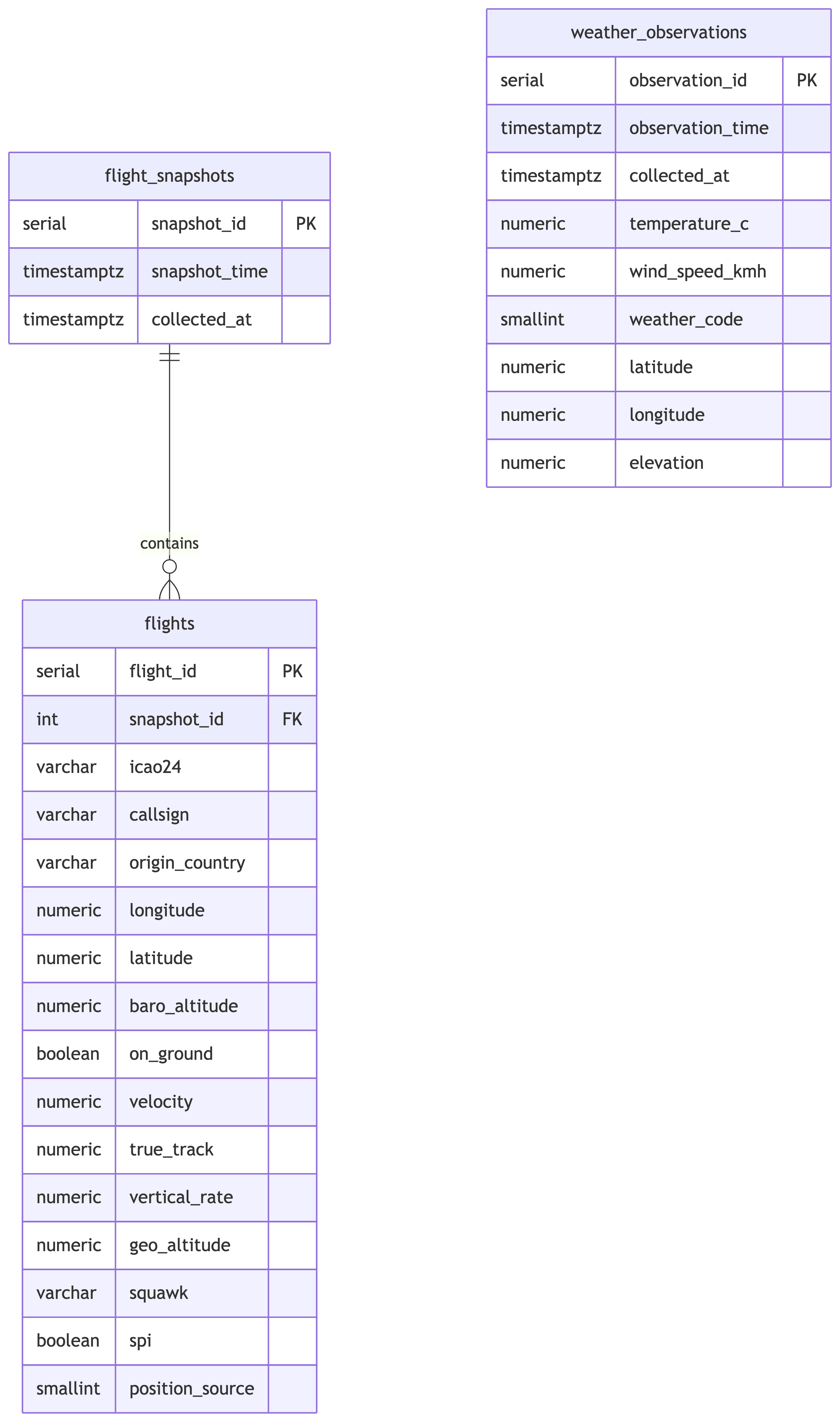
Why Two Flight Tables?
Each API call returns one timestamp and many aircraft. That is a classic one-to-many relationship:
- flight_snapshots: one row per API call (the “when”)
- flights: one row per aircraft per snapshot (the “what”)
If we jammed everything into one table, we would duplicate the snapshot timestamp for every aircraft. That is denormalized, and we just spent three weeks learning why that is bad.
Design Decisions
flight_snapshots
snapshot_timecomes from the JSON (raw_json->>'time'), converted from Unix epochcollected_atcomes from the staging table’screated_atcolumn- These are usually close but not identical. The API timestamp tells us when OpenSky gathered the data; our timestamp tells us when we grabbed it.
flights
- Each field maps to an array index (0-16) in the state vector
- Callsigns are trimmed of trailing whitespace
- Nullable fields (
baro_altitude,vertical_rate,geo_altitude,squawk) stay nullable
weather_observations
- Flat table since each observation is a single data point, no arrays to normalize
observation_timeparsed from the ISO timestamp in the JSON- We keep
latitude,longitude,elevationeven though they are constant, because good schema design does not assume things stay constant
The DDL
CREATE TABLE flight_snapshots (
    snapshot_id serial PRIMARY KEY,
    snapshot_time timestamptz NOT NULL,
    collected_at timestamptz NOT NULL
);

CREATE TABLE flights (
    flight_id serial PRIMARY KEY,
    snapshot_id int NOT NULL REFERENCES flight_snapshots(snapshot_id),
    icao24 varchar(10),
    callsign varchar(10),
    origin_country varchar(100),
    longitude numeric(9,4),
    latitude numeric(8,4),
    baro_altitude numeric(8,2),
    on_ground boolean,
    velocity numeric(7,2),
    true_track numeric(6,2),
    vertical_rate numeric(6,2),
    geo_altitude numeric(8,2),
    squawk varchar(10),
    spi boolean,
    position_source smallint
);

CREATE TABLE weather_observations (
    observation_id serial PRIMARY KEY,
    observation_time timestamptz NOT NULL,
    collected_at timestamptz NOT NULL,
    temperature_c numeric(5,2),
    wind_speed_kmh numeric(6,2),
    weather_code smallint,
    latitude numeric(8,4),
    longitude numeric(9,4),
    elevation numeric(6,1)
);
Your data finally looks like it was entered by someone who cares.
Part 4: The Transform Step
This is where the magic happens. We take the JSON blobs and extract structured, typed, normalized rows.
Think of it as the database equivalent of unpacking after a move and actually putting things in drawers.
Migrating JSON to Relational Tables
Step 1: Populate flight_snapshots
Each row in flight_json_data becomes one row in flight_snapshots. We convert the Unix timestamp to a proper timestamptz:
The DISTINCT handles any duplicate snapshots. The to_timestamp() function converts Unix epoch seconds into a PostgreSQL timestamp. No more staring at 1772503243 and wondering what day that is.
Step 2: Populate flights
This is the big one. We unnest the state arrays and join back to flight_snapshots to get the foreign key:
INSERT INTO flights (
    snapshot_id, icao24, callsign, origin_country,
    longitude, latitude, baro_altitude, on_ground,
    velocity, true_track, vertical_rate, geo_altitude,
    squawk, spi, position_source
)
SELECT
    fs.snapshot_id,
    state->>0 AS icao24,
    TRIM(state->>1) AS callsign,
    state->>2 AS origin_country,
    (state->>5)::numeric AS longitude,
    (state->>6)::numeric AS latitude,
    (state->>7)::numeric AS baro_altitude,
    (state->>8)::boolean AS on_ground,
    (state->>9)::numeric AS velocity,
    (state->>10)::numeric AS true_track,
    (state->>11)::numeric AS vertical_rate,
    (state->>13)::numeric AS geo_altitude,
    state->>14 AS squawk,
    (state->>15)::boolean AS spi,
    (state->>16)::smallint AS position_source
FROM flight_json_data fjd
JOIN flight_snapshots fs
    ON to_timestamp((fjd.raw_json->>'time')::bigint) = fs.snapshot_time
CROSS JOIN jsonb_array_elements(fjd.raw_json->'states') AS state
WHERE fjd.raw_json->'states' IS NOT NULL
    AND fjd.raw_json->>'states' != 'null';
Let’s break down what is happening:
CROSS JOIN jsonb_array_elements(...)unnests each aircraft array into its own row- We join back to
flight_snapshotsto get thesnapshot_idforeign key - The
WHEREclause filters out snapshots with no aircraft - Array indices 0-16 map to the state vector positions we documented earlier
- Notice index 12 (sensors) is skipped since it is almost always null and not useful for analysis
Step 3: Populate weather_observations
Weather is straightforward since there is no array to unnest:
INSERT INTO weather_observations (
    observation_time, collected_at,
    temperature_c, wind_speed_kmh, weather_code,
    latitude, longitude, elevation
)
SELECT
    (raw_json->'current'->>'time')::timestamptz AS observation_time,
    created_at AS collected_at,
    (raw_json->'current'->>'temperature_2m')::numeric AS temperature_c,
    (raw_json->'current'->>'wind_speed_10m')::numeric AS wind_speed_kmh,
    (raw_json->'current'->>'weathercode')::smallint AS weather_code,
    (raw_json->>'latitude')::numeric AS latitude,
    (raw_json->>'longitude')::numeric AS longitude,
    (raw_json->>'elevation')::numeric AS elevation
FROM weather_json_data
WHERE raw_json->'current' IS NOT NULL;
Verification Queries
Always verify your transforms. Trust, but verify. Actually, just verify.
-- How many snapshots?
SELECT count(*) FROM flight_snapshots;

-- How many individual flight records?
SELECT count(*) FROM flights;

-- How many weather observations?
SELECT count(*) FROM weather_observations;

-- Spot check: flights per snapshot
SELECT fs.snapshot_id,
       fs.snapshot_time,
       count(f.flight_id) AS num_flights
FROM flight_snapshots fs
LEFT JOIN flights f ON fs.snapshot_id = f.snapshot_id
GROUP BY fs.snapshot_id, fs.snapshot_time
ORDER BY num_flights DESC
LIMIT 10;

-- Spot check: weather range
SELECT
    min(temperature_c) AS min_temp,
    max(temperature_c) AS max_temp,
    min(wind_speed_kmh) AS min_wind,
    max(wind_speed_kmh) AS max_wind,
    min(observation_time) AS earliest,
    max(observation_time) AS latest
FROM weather_observations;
If your flight count is zero, go back and check your WHERE clause. If your temperature range includes 500 degrees Celsius, something went very wrong with your casting.
Part 5: Railway Transform Service
You do not want to run these transforms by hand every time new data comes in. Let’s automate it.
Deploying Transforms on Railway
The db_transform Template
Clone the template repo:
https://github.com/LucasCordova/db_transformThis repo contains a simple setup:
- A
Dockerfilethat runs a SQL file against your Postgres database - A
clean.sqlfile where you put your transform queries - That is it. No frameworks, no dependencies, no opinions.
You put your SQL in clean.sql, deploy to Railway, and it runs.
Step-by-Step Deployment
Fork or clone the
db_transformrepo to your own GitHub accountEdit
clean.sqlwith the transform queries from Part 4 (insert-select, etc.)Commit and push to your GitHub repo
In Railway dashboard, click “New” then “GitHub Repo”
Select your repo from the list
Add the
DATABASE_URLenvironment variable pointing to your Railway Postgres instance (find this in your Postgres service’s Variables tab)Deploy and the service runs
clean.sqlagainst your databaseOptional: Set up as a cron job in Railway for recurring transforms
What Does “Idempotent” Mean?
An operation is idempotent if running it once or a hundred times produces the same result. The first run changes things. Every run after that changes nothing.
| Statement | Idempotent? | Why |
|---|---|---|
CREATE TABLE IF NOT EXISTS |
Yes | First run creates it, subsequent runs skip it |
CREATE TABLE |
No | Second run errors because the table already exists |
TRUNCATE then INSERT |
Yes | Every run wipes and rebuilds, same result every time |
Just INSERT |
No | Every run adds more duplicate rows |
This matters because your cron transform runs repeatedly. If your clean.sql is not idempotent, you get duplicate data piling up every cycle. If it is idempotent, it does not matter if it runs once or fifty times. Same clean dataset every time.
Important Notes on the Transform Service
- The service runs once and exits. It is not a long-running server.
- If you need to re-run, trigger a new deployment or use Railway’s cron feature.
- Make your SQL idempotent. Since the cron runs repeatedly against a database that keeps accumulating new staging data, you need to avoid inserting duplicate rows every time.
- The
DATABASE_URLenvironment variable is automatically available inside the container.
Important Notes on the Transform Service (continued)
The key pattern: truncate your target tables before re-inserting. Your staging tables (flight_json_data, weather_json_data) keep growing as the API scrapers add rows. Each cron run should wipe the transformed tables and rebuild them from the full staging dataset.
-- ============================================================
-- clean.sql - Idempotent transform for Railway cron
-- This runs on every cron trigger. It rebuilds the
-- normalized tables from scratch using the staging data.
-- ============================================================

-- Step 1: Create tables if they do not exist yet (first run)
CREATE TABLE IF NOT EXISTS flight_snapshots (
    snapshot_id serial PRIMARY KEY,
    snapshot_time timestamptz NOT NULL,
    collected_at timestamptz NOT NULL
);

CREATE TABLE IF NOT EXISTS flights (
    flight_id serial PRIMARY KEY,
    snapshot_id integer REFERENCES flight_snapshots (snapshot_id),
    icao24 varchar(10),
    callsign varchar(10),
    origin_country varchar(100),
    longitude numeric(9,4),
    latitude numeric(8,4),
    baro_altitude numeric(8,2),
    on_ground boolean,
    velocity numeric(7,2),
    true_track numeric(6,2),
    vertical_rate numeric(6,2),
    geo_altitude numeric(8,2),
    squawk varchar(10),
    spi boolean,
    position_source smallint
);

CREATE TABLE IF NOT EXISTS weather_observations (
    observation_id serial PRIMARY KEY,
    observation_time timestamptz NOT NULL,
    collected_at timestamptz NOT NULL,
    temperature_c numeric(5,2),
    wind_speed_kmh numeric(6,2),
    weather_code smallint,
    latitude numeric(8,4),
    longitude numeric(9,4),
    elevation numeric(6,1)
);

-- Step 2: Truncate in dependency order (children first)
-- RESTART IDENTITY resets the serial counters
-- CASCADE is not needed here because we truncate children first,
-- but it is a safety net
TRUNCATE flights RESTART IDENTITY;
TRUNCATE flight_snapshots RESTART IDENTITY CASCADE;
TRUNCATE weather_observations RESTART IDENTITY;

-- Step 3: Re-populate from staging data
-- (same INSERT INTO ... SELECT queries from the transform step)

-- Weather observations
INSERT INTO weather_observations (
    observation_time, collected_at, temperature_c,
    wind_speed_kmh, weather_code,
    latitude, longitude, elevation
)
SELECT DISTINCT
    (raw_json->'current'->>'time')::timestamptz,
    created_at,
    (raw_json->'current'->>'temperature_2m')::numeric,
    (raw_json->'current'->>'wind_speed_10m')::numeric,
    (raw_json->'current'->>'weathercode')::smallint,
    (raw_json->>'latitude')::numeric,
    (raw_json->>'longitude')::numeric,
    (raw_json->>'elevation')::numeric
FROM weather_json_data;

-- Flight snapshots (only rows where states is not null)
INSERT INTO flight_snapshots (snapshot_time, collected_at)
SELECT DISTINCT
    to_timestamp((raw_json->>'time')::bigint),
    created_at
FROM flight_json_data
WHERE raw_json->'states' IS NOT NULL
  AND raw_json->>'states' != 'null';

-- Flights (unnest the states array)
INSERT INTO flights (
    snapshot_id, icao24, callsign, origin_country,
    longitude, latitude, baro_altitude, on_ground,
    velocity, true_track, vertical_rate,
    geo_altitude, squawk, spi, position_source
)
SELECT
    fs.snapshot_id,
    trim(state->>0),
    trim(state->>1),
    state->>2,
    (state->>5)::numeric,
    (state->>6)::numeric,
    (state->>7)::numeric,
    (state->>8)::boolean,
    (state->>9)::numeric,
    (state->>10)::numeric,
    (state->>11)::numeric,
    (state->>13)::numeric,
    state->>14,
    (state->>15)::boolean,
    (state->>16)::smallint
FROM flight_json_data f
JOIN flight_snapshots fs
    ON to_timestamp((f.raw_json->>'time')::bigint) = fs.snapshot_time
CROSS JOIN jsonb_array_elements(f.raw_json->'states') AS state
WHERE f.raw_json->'states' IS NOT NULL
  AND f.raw_json->>'states' != 'null';
Important Notes on the Transform Service (continued)
Every time the cron fires, this wipes the normalized tables and rebuilds them from whatever is currently in the staging tables. New API data that arrived since the last run gets included automatically. This is the nuclear-but-reliable approach: no partial states, no duplicate rows, no “did that row already get transformed?” headaches.
For large datasets where a full rebuild is too slow, you would instead track a high-water mark (e.g., the max id or created_at you last processed) and only transform new rows. But for our dataset size, the full truncate-and-reload is perfectly fine and much simpler to reason about.
Part 6: Advanced Statistics in SQL
Now the fun part. We have clean, normalized data. Time to interrogate it.
Research Question: Does weather affect the volume and behavior of air traffic over Portland?
Descriptive Statistics
Getting Our Bearings
Before we correlate anything, we need to know what “normal” looks like. Descriptive statistics give us the baseline.
-- Flight counts per snapshot
SELECT
    count(*) AS num_snapshots,
    round(avg(flight_count), 2) AS avg_flights,
    round(stddev_pop(flight_count), 2) AS stddev_flights,
    min(flight_count) AS min_flights,
    max(flight_count) AS max_flights
FROM (
    SELECT fs.snapshot_id,
           count(f.flight_id) AS flight_count
    FROM flight_snapshots fs
    LEFT JOIN flights f ON fs.snapshot_id = f.snapshot_id
    GROUP BY fs.snapshot_id
) sub;
This tells us the average number of aircraft visible over Portland at any given moment, plus how much that varies.
Weather Descriptive Stats
-- Temperature and wind statistics
SELECT
    count(*) AS num_observations,
    round(avg(temperature_c), 2) AS avg_temp_c,
    round(stddev_pop(temperature_c), 2) AS stddev_temp,
    round(min(temperature_c), 2) AS min_temp,
    round(max(temperature_c), 2) AS max_temp,
    round(avg(wind_speed_kmh), 2) AS avg_wind,
    round(stddev_pop(wind_speed_kmh), 2) AS stddev_wind,
    round(min(wind_speed_kmh), 2) AS min_wind,
    round(max(wind_speed_kmh), 2) AS max_wind
FROM weather_observations;
Flight Altitude Statistics
-- Altitude statistics for airborne aircraft
SELECT
    count(*) AS num_airborne,
    round(avg(baro_altitude), 2) AS avg_altitude_m,
    round(stddev_pop(baro_altitude), 2) AS stddev_altitude,
    round(min(baro_altitude), 2) AS min_altitude,
    round(max(baro_altitude), 2) AS max_altitude,
    round(avg(velocity), 2) AS avg_speed_ms,
    round(stddev_pop(velocity), 2) AS stddev_speed
FROM flights
WHERE on_ground = false
    AND baro_altitude IS NOT NULL;
If the standard deviation of altitude is enormous, that just means we are seeing everything from small Cessnas at 500 meters to commercial jets at 10,000 meters. Portland airspace is busy.
Views
What is a View?
A view is a saved SQL query that acts like a virtual table. It does not store data – it is just a named SELECT statement that lives in the database.
Every time you query a view, PostgreSQL runs the underlying query fresh against the actual tables.
No duplicate data. No extra storage. Just a query with a name.
Why Use Views?
Simplify complex queries. A gnarly 15-line JOIN with filters becomes SELECT * FROM that_view. The complexity lives in one place.
Abstraction layer. If the underlying table structure changes, update the view definition. Downstream queries do not break.
Security and access control. Grant someone access to a view that shows only certain columns or rows, without exposing the full table. Think: employees seeing their own records but not everyone else’s salaries.
Reusability. Same complex query used in 5 different reports? One view, five simple queries.
When to Use Views (and When Not To)
Use views when:
- You are writing the same JOIN/filter combo repeatedly
- You need to restrict what users can see
- You want meaningful names for derived datasets (
monthly_revenuebeats a sprawling subquery) - You are building a reporting layer on top of a normalized schema
When to Use Views (and When Not To)
Do not use views when:
- You need cached/precomputed results (that is a materialized view, a different thing)
- The query is a simple one-off you will run once
- You are nesting views on views on views (gets hard to debug fast)
Creating the Hourly Analysis View
For meaningful statistics, we need to aggregate to a common time grain. Five-minute snapshots are too noisy. Let’s use hourly buckets:
-- Hourly flight counts
CREATE OR REPLACE VIEW hourly_flights AS
SELECT
    date_trunc('hour', fs.snapshot_time) AS hour,
    count(DISTINCT fs.snapshot_id) AS num_snapshots,
    count(f.flight_id) AS total_flights,
    round(count(f.flight_id)::numeric
        / NULLIF(count(DISTINCT fs.snapshot_id), 0), 2) AS avg_flights_per_snapshot
FROM flight_snapshots fs
LEFT JOIN flights f ON fs.snapshot_id = f.snapshot_id
GROUP BY date_trunc('hour', fs.snapshot_time);

-- Hourly weather (average across observations in each hour)
CREATE OR REPLACE VIEW hourly_weather AS
SELECT
    date_trunc('hour', observation_time) AS hour,
    round(avg(temperature_c), 2) AS avg_temp_c,
    round(avg(wind_speed_kmh), 2) AS avg_wind_kmh,
    mode() WITHIN GROUP (ORDER BY weather_code) AS predominant_weather_code
FROM weather_observations
GROUP BY date_trunc('hour', observation_time);

-- Combined hourly view for correlation analysis
CREATE OR REPLACE VIEW hourly_flight_weather AS
SELECT
    hf.hour,
    hf.num_snapshots,
    hf.total_flights,
    hf.avg_flights_per_snapshot,
    hw.avg_temp_c,
    hw.avg_wind_kmh,
    hw.predominant_weather_code
FROM hourly_flights hf
JOIN hourly_weather hw ON hf.hour = hw.hour;
These views align our flight and weather data on the same hourly grid. This is how you join data that was collected independently at different intervals. Round to a common grain, then join on it.
Correlation
corr(Y, X): Measuring Linear Relationships
The corr() function returns the Pearson correlation coefficient, a value between -1 and +1:
| Value | Meaning |
|---|---|
| +1.0 | Perfect positive correlation |
| 0.0 | No linear relationship |
| -1.0 | Perfect negative correlation |
Anything above 0.7 or below -0.7 is strong. Between 0.3 and 0.7 is moderate. Below 0.3 is weak or nonexistent.
Temperature vs. Flight Volume
If this is positive, warmer hours tend to have more flights. Makes intuitive sense: better weather, more VFR (visual flight rules) traffic, more general aviation.
Wind Speed vs. Flight Behavior
-- Does wind speed affect average altitude or ground speed?
SELECT
    round(corr(avg_alt, avg_wind_kmh)::numeric, 4) AS wind_altitude_corr,
    round(corr(avg_speed, avg_wind_kmh)::numeric, 4) AS wind_speed_corr
FROM (
    SELECT
        hw.hour,
        hw.avg_wind_kmh,
        avg(f.baro_altitude) AS avg_alt,
        avg(f.velocity) AS avg_speed
    FROM hourly_weather hw
    JOIN flight_snapshots fs
        ON date_trunc('hour', fs.snapshot_time) = hw.hour
    JOIN flights f ON fs.snapshot_id = f.snapshot_id
    WHERE f.on_ground = false
        AND f.baro_altitude IS NOT NULL
    GROUP BY hw.hour, hw.avg_wind_kmh
) sub;
A positive correlation between wind and altitude could mean pilots climb higher to find smoother air. Or it could mean nothing. We will get to that.
Wind Speed vs. Flight Volume
If this is negative, windier conditions correlate with fewer flights. Small aircraft stay grounded in high winds, so we might see this in the data.
Regression
Linear Regression in SQL
Correlation tells you there is a relationship. Regression tells you the equation.
| Function | Returns |
|---|---|
regr_slope(Y, X) |
Slope of the regression line |
regr_intercept(Y, X) |
Y-intercept |
regr_r2(Y, X) |
R-squared (how well the line fits) |
The formula: Y = slope * X + intercept
R-squared ranges from 0 to 1. An R-squared of 0.8 means the model explains 80% of the variance. An R-squared of 0.05 means your model explains almost nothing and you should probably find a better predictor.
Predicting Flight Volume from Temperature
Read the slope as: “For each 1 degree C increase in temperature, we expect X more flights per hour.”
The R-squared tells us how much of the variation in flight volume is explained by temperature alone. Spoiler: probably not a lot, because many other factors affect air traffic.
Predicting Flight Volume from Wind Speed
If the slope is negative and R-squared is low, wind matters a little but is far from the whole story. Time of day, day of week, and airline schedules all matter more than a light breeze.
Window Functions
The Problem with GROUP BY
GROUP BY is powerful, but it has a fundamental limitation: it collapses rows. You get one output row per group, and you lose access to individual rows.
What if you want the count and still see every individual flight? You cannot. GROUP BY forces a choice: aggregated summary or individual detail. Never both.
Window Functions: The Best of Both Worlds
A window function performs a calculation across a set of rows that are somehow related to the current row – without collapsing them.
Every row keeps its individual data. But each row also gets the overall average altitude attached to it. No grouping. No collapsing. Every row survives.
The OVER() clause is what makes a function a window function. It defines the “window” of rows the function looks at.
How Window Functions Work
Think of it as a sliding lens over your result set:
- PostgreSQL computes the full result set first
- For each row, it looks through the “window” defined by
OVER() - It computes the function across that window
- It attaches the result to the current row
- It moves to the next row and repeats
The key insight: the original rows are never collapsed. You get computation across rows while keeping every row intact.
The OVER() Clause
OVER() controls what the window function can see:
| Clause | What It Does | Example |
|---|---|---|
OVER () |
Entire result set is the window | Global average across all rows |
OVER (ORDER BY col) |
Running calculation in that order | Cumulative sum, ranking |
OVER (PARTITION BY col) |
Separate window per group | Average per department |
OVER (PARTITION BY a ORDER BY b) |
Ordered calculation within groups | Rank within each category |
-- Global: one window for everything
sum(total_flights) OVER ()

-- Partitioned: separate window per weather code
sum(total_flights) OVER (PARTITION BY weather_code)

-- Ordered: running total in time order
sum(total_flights) OVER (ORDER BY hour)

-- Both: running total within each weather code
sum(total_flights) OVER (
    PARTITION BY weather_code ORDER BY hour
)
Window Functions vs GROUP BY
| GROUP BY | Window Function | |
|---|---|---|
| Rows | Collapsed into groups | Preserved individually |
| Output | One row per group | Same number of rows as input |
| Access | Only grouped/aggregated columns | All columns plus computed values |
| Use case | Summaries and reports | Analysis alongside detail |
You will often use both in the same query: GROUP BY to aggregate to the grain you need, then window functions on top to rank or compare those aggregates.
Types of Window Functions
Aggregate window functions – familiar aggregates with OVER():
sum(),avg(),count(),min(),max()
Ranking functions – assign positions:
rank(),dense_rank(),row_number(),ntile()
Value functions – access other rows:
lag()(previous row),lead()(next row)first_value(),last_value(),nth_value()
All of them use OVER(). That is the unifying syntax. If you see OVER(), you are looking at a window function.
Ranking
Why Rank Data?
Sorting gives you order. Ranking gives you position.
Sometimes you do not just want to see rows ordered by value – you want to know where each row stands relative to the others. That is a fundamentally different question.
- “What were the busiest hours?” – sorting works fine
- “Was this hour in the top 10 busiest?” – you need a rank
- “Was this the busiest hour for a Tuesday?” – you need a rank within a group
Ranking is how you go from “show me the data” to “show me how the data compares to itself.”
When to Use Ranking
Leaderboards and top-N analysis. Find the top 5 airports, the bottom 10 performing stores, the highest-scoring students. You could use ORDER BY ... LIMIT, but ranking lets you keep all the data while labeling positions.
Comparisons within groups. “Rank each employee’s sales within their department.” This is PARTITION BY department ORDER BY sales – every department gets its own ranking starting at 1.
Handling ties explicitly. When two rows have the same value, do you skip the next number or not? ORDER BY does not answer this. Ranking functions do.
Filtering by position. Wrap a ranking query in a subquery or CTE, then filter: WHERE rank <= 3. You cannot do this with plain ORDER BY because rank is computed, not stored.
The Three Ranking Functions
| Function | Behavior on Ties | Example (4 rows, tie at #2) |
|---|---|---|
rank() |
Same rank for ties, skip next | 1, 2, 2, 4 |
dense_rank() |
Same rank for ties, no skip | 1, 2, 2, 3 |
row_number() |
No ties ever, arbitrary tiebreak | 1, 2, 3, 4 |
Use rank() when gaps matter (sports standings, competition results).
Use dense_rank() when you want consecutive numbers (top-3 means exactly 3 distinct ranks, even with ties).
Use row_number() when you need unique row identifiers or want to pick one arbitrary winner per group.
All three use the OVER(ORDER BY ...) clause. Add PARTITION BY to rank within groups.
The OVER() Clause
The OVER() clause is what makes these window functions. It defines:
- ORDER BY – what determines rank position
- PARTITION BY (optional) – restart ranking for each group
Without PARTITION BY, every row competes against every other row. With it, each group gets its own independent ranking. Think of it as running a separate ORDER BY for each group, then stitching the results back together.
Ranking Hours by Flight Volume
The busiest hours will likely be mid-afternoon on weekdays. That is when commercial traffic peaks and general aviation is most active.
Ranking by Altitude Within Weather Conditions
-- Rank hours by average altitude, partitioned by weather code
SELECT
    hw.hour,
    hw.predominant_weather_code,
    round(avg(f.baro_altitude), 2) AS avg_altitude,
    dense_rank() OVER (
        PARTITION BY hw.predominant_weather_code
        ORDER BY avg(f.baro_altitude) DESC
    ) AS altitude_rank
FROM hourly_weather hw
JOIN flight_snapshots fs
    ON date_trunc('hour', fs.snapshot_time) = hw.hour
JOIN flights f ON fs.snapshot_id = f.snapshot_id
WHERE f.on_ground = false
    AND f.baro_altitude IS NOT NULL
GROUP BY hw.hour, hw.predominant_weather_code
ORDER BY hw.predominant_weather_code, altitude_rank
LIMIT 20;
PARTITION BY weather_code restarts the ranking for each weather condition. This lets us compare altitude rankings within clear weather separately from overcast conditions.
Top Flight Hours by Day of Week
-- Rank flight volume within each day of week
SELECT
    to_char(hour, 'Day') AS day_of_week,
    extract(hour FROM hour) AS hour_of_day,
    total_flights,
    rank() OVER (
        PARTITION BY extract(dow FROM hour)
        ORDER BY total_flights DESC
    ) AS rank_within_day
FROM hourly_flight_weather
ORDER BY extract(dow FROM hour), rank_within_day
LIMIT 20;
Rolling Averages
Window Functions with Frame Clauses
Rolling averages smooth out noisy data so you can see trends. The syntax:
This computes the average of the current row plus 3 rows before and 3 rows after, giving a 7-row moving average. Change the numbers to adjust the smoothing window.
Rolling Average of Flight Volume
-- 6-hour rolling average of flights (3 hours before, 3 after)
SELECT
    hour,
    total_flights,
    round(avg(total_flights) OVER (
        ORDER BY hour
        ROWS BETWEEN 3 PRECEDING AND 3 FOLLOWING
    ), 2) AS rolling_avg_flights,
    avg_temp_c,
    round(avg(avg_temp_c) OVER (
        ORDER BY hour
        ROWS BETWEEN 3 PRECEDING AND 3 FOLLOWING
    ), 2) AS rolling_avg_temp
FROM hourly_flight_weather
ORDER BY hour;
The raw total_flights column will be spiky. The rolling average smooths it out so you can see whether flight volume trends up during the day and down at night. Which it will, unless Portland’s airport has gone rogue.
Comparing Raw vs. Smoothed Data
-- Show the difference between raw and smoothed values
SELECT
    hour,
    total_flights AS raw,
    round(avg(total_flights) OVER (
        ORDER BY hour
        ROWS BETWEEN 6 PRECEDING AND 6 FOLLOWING
    ), 2) AS smoothed_12hr,
    total_flights - round(avg(total_flights) OVER (
        ORDER BY hour
        ROWS BETWEEN 6 PRECEDING AND 6 FOLLOWING
    ), 2) AS residual
FROM hourly_flight_weather
ORDER BY hour;
The residual column shows how much each hour deviates from its local trend. Large positive residuals are unusually busy hours. Large negative residuals are unusually quiet. These outliers are often the most interesting data points.
Cumulative Flights Over Time
This gives you a sense of how data has been accumulating over the two weeks. If there is a flat spot, your scraper probably went down. If there is a sudden jump, you caught a busy travel day.
Rates and Comparisons
Calculating Meaningful Rates
Raw counts are not always comparable. Flights at 3 AM vs. 3 PM are different contexts. Rates normalize the data so comparisons make sense.
-- Average flights per hour by time of day
SELECT
    extract(hour FROM hour) AS hour_of_day,
    count(*) AS num_observations,
    round(avg(total_flights), 2) AS avg_flights,
    round(stddev_pop(total_flights), 2) AS stddev_flights
FROM hourly_flight_weather
GROUP BY extract(hour FROM hour)
ORDER BY hour_of_day;
This shows the daily rhythm of Portland air traffic. Expect a dip in the early morning hours and peaks in the afternoon.
CASE Statements
What is a CASE Statement?
A CASE statement is SQL’s version of if/else. It lets you create new values based on conditions, right inside a query.
PostgreSQL evaluates the WHEN conditions top to bottom. The first one that is true wins. If none match, ELSE is returned. If there is no ELSE and nothing matches, you get NULL.
Two Forms of CASE
Searched CASE – each WHEN has its own condition (most flexible):
Simple CASE – compares one expression against values (cleaner for equality checks):
Use simple CASE when you are matching one column against specific values. Use searched CASE when you need ranges, multiple columns, or complex logic.
Where Can You Use CASE?
Anywhere you can put an expression:
- SELECT – create computed columns (most common)
- WHERE – conditional filtering
- GROUP BY – group by computed categories
- ORDER BY – custom sort orders
- Inside aggregates – conditional counting
This pattern – CASE inside an aggregate – is one of the most useful tricks in SQL. It lets you pivot categories into columns without a pivot table.
CASE in GROUP BY
When you use CASE in a SELECT and want to group by it, you have to repeat the full expression in the GROUP BY clause. PostgreSQL does not let you reference a column alias in GROUP BY.
SELECT
    CASE
        WHEN wind_speed_kmh > 30 THEN 'High wind'
        WHEN wind_speed_kmh > 15 THEN 'Moderate wind'
        ELSE 'Low wind'
    END AS wind_category,
    count(*) AS num_observations,
    round(avg(temperature_c), 2) AS avg_temp
FROM weather_observations
GROUP BY
    CASE
        WHEN wind_speed_kmh > 30 THEN 'High wind'
        WHEN wind_speed_kmh > 15 THEN 'Moderate wind'
        ELSE 'Low wind'
    END;
Yes, you write it twice. It is annoying. A CTE or subquery can avoid the repetition if it bothers you.
Weekday vs. Weekend Traffic
-- Compare weekday and weekend flight volumes
SELECT
    CASE
        WHEN extract(dow FROM hour) IN (0, 6) THEN 'Weekend'
        ELSE 'Weekday'
    END AS day_type,
    count(*) AS num_hours,
    round(avg(total_flights), 2) AS avg_flights_per_hour,
    round(stddev_pop(total_flights), 2) AS stddev_flights,
    round(avg(avg_temp_c), 2) AS avg_temp,
    round(avg(avg_wind_kmh), 2) AS avg_wind
FROM hourly_flight_weather
GROUP BY
    CASE
        WHEN extract(dow FROM hour) IN (0, 6) THEN 'Weekend'
        ELSE 'Weekday'
    END;
If weekday traffic is significantly higher, that is commercial aviation at work. If weekend traffic is comparable, Portland’s general aviation community is active.
Flight Rate by Weather Condition
-- Average flights per hour grouped by weather code
SELECT
    predominant_weather_code,
    CASE predominant_weather_code
        WHEN 0 THEN 'Clear'
        WHEN 1 THEN 'Mainly clear'
        WHEN 2 THEN 'Partly cloudy'
        WHEN 3 THEN 'Overcast'
        WHEN 45 THEN 'Fog'
        WHEN 51 THEN 'Light drizzle'
        WHEN 53 THEN 'Moderate drizzle'
        WHEN 55 THEN 'Dense drizzle'
        WHEN 61 THEN 'Light rain'
        WHEN 63 THEN 'Moderate rain'
        WHEN 65 THEN 'Heavy rain'
        ELSE 'Other (' || predominant_weather_code || ')'
    END AS weather_description,
    count(*) AS num_hours,
    round(avg(total_flights), 2) AS avg_flights,
    round(avg(avg_wind_kmh), 2) AS avg_wind
FROM hourly_flight_weather
GROUP BY predominant_weather_code
ORDER BY avg_flights DESC;
This is the most direct answer to our research question. If “Clear” has significantly more flights than “Moderate rain,” weather matters. If they are similar, Portland pilots just do not care about rain. Which, honestly, tracks.
Putting It All Together: Multi-Factor Analysis
-- Combine temperature bins, wind bins, and weather code
SELECT
    CASE
        WHEN avg_temp_c < 5 THEN 'Cold (<5C)'
        WHEN avg_temp_c < 10 THEN 'Cool (5-10C)'
        WHEN avg_temp_c < 15 THEN 'Mild (10-15C)'
        ELSE 'Warm (>15C)'
    END AS temp_bin,
    CASE
        WHEN avg_wind_kmh < 10 THEN 'Calm (<10 km/h)'
        WHEN avg_wind_kmh < 20 THEN 'Breezy (10-20 km/h)'
        ELSE 'Windy (>20 km/h)'
    END AS wind_bin,
    count(*) AS num_hours,
    round(avg(total_flights), 2) AS avg_flights,
    round(avg(avg_flights_per_snapshot), 2) AS avg_per_snapshot
FROM hourly_flight_weather
GROUP BY
    CASE
        WHEN avg_temp_c < 5 THEN 'Cold (<5C)'
        WHEN avg_temp_c < 10 THEN 'Cool (5-10C)'
        WHEN avg_temp_c < 15 THEN 'Mild (10-15C)'
        ELSE 'Warm (>15C)'
    END,
    CASE
        WHEN avg_wind_kmh < 10 THEN 'Calm (<10 km/h)'
        WHEN avg_wind_kmh < 20 THEN 'Breezy (10-20 km/h)'
        ELSE 'Windy (>20 km/h)'
    END
ORDER BY avg_flights DESC;
This crosstab shows flight volume for every combination of temperature and wind conditions. If “Warm + Calm” consistently has the most flights and “Cold + Windy” has the fewest, we have a clear pattern.
Part 7: Answering the Research Question
What Did We Find?
The Verdict
Research Question: Does weather affect the volume and behavior of air traffic over Portland?
Based on our analysis:
Temperature and flight volume: Likely a weak-to-moderate positive correlation. Warmer hours have somewhat more flights, but time of day is a massive confound since it is warmer during the day when more flights operate anyway.
Wind speed and flight volume: Likely a weak negative correlation. Very windy hours may have slightly fewer flights, but Portland rarely gets wind severe enough to ground commercial aviation.
Weather code and flight volume: Probably the strongest signal. Clear vs. rainy conditions may show meaningful differences, especially for general aviation traffic.
The elephant in the room: Time of day and airline schedules dominate flight patterns far more than weather does in two weeks of March data.
Correlation Is Not Causation
This bears repeating every time you run corr():
- Correlation measures linear association, not cause and effect
- Temperature correlates with flight volume, but temperature does not cause flights to take off
- Both are driven by time of day (confounding variable)
- To truly isolate weather effects, you would need to control for time of day, day of week, and seasonal patterns
Two weeks of data in March is a starting point, not a conclusion. A full year of data across all seasons would give us much more to work with.
Where Do We Go From Here?
Coming Up Next
We have a normalized database. We have views that answer real questions. We have statistical analysis that tells a story. But right now, only people who know SQL can access any of it.
That changes next.
API Service over PostgreSQL. We will build a REST API that sits on top of our database, so other developers can query our flight and weather data over HTTP without writing SQL. Your database becomes a service that anyone can consume – a web app, a mobile app, another team’s pipeline.
Dashboards with Grafana. We will connect Grafana directly to our PostgreSQL database and build interactive dashboards on top of our queries and views. Instead of running SQL and reading result tables, you will have live charts and graphs that update as new data flows in.
The Big Picture
Scrapers (Railway)
    |
    v
PostgreSQL Database
    |
    +--> Views & Queries (what we built today)
    |
    +--> REST API --> Other developers, apps, pipelines
    |
    +--> Grafana Dashboard --> Visual monitoring & analysis
Your project will be become (hopefully!) a complete data platform: collection, storage, transformation, analysis, access, and visualization. That is data engineering.
References
- DeBarros, A. (2022). Practical SQL: A Beginner’s Guide to Storytelling with Data (2nd ed.). No Starch Press. Chapter 11.
- OpenSky Network API: https://openskynetwork.github.io/opensky-api/
- Open-Meteo API: https://open-meteo.com/en/docs
- WMO Weather Codes: https://www.nodc.noaa.gov/archive/arc0021/0002199/1.1/data/0-data/HTML/WMO-CODE/WMO4677.HTM
- PostgreSQL Aggregate Functions: https://www.postgresql.org/docs/current/functions-aggregate.html