Lecture 10-2: Working with Dates and Times

DATA 503: Fundamentals of Data Engineering

Lucas P. Cordova, Ph.D.

lpcordova@willamette.edu

Willamette University

March 16, 2026

Lecture Outline

• Part 1: Setting Up
• Part 2: Date and Time Data Types
• Part 3: Extracting Date and Time Components
• Part 4: Creating Dates and Times
• Part 5: Time Zones
• Part 6: Date and Time Math
• Part 7: NYC Taxi Trip Analysis
• Part 8: Amtrak Train Trips
• Part 9: CTEs and Useful PostgreSQL Features
• Part 10: Putting It All Together (Exercises)
• Part 11: What We Learned

Part 1: Setting Up

Before we start manipulating time itself, we need to load some data.

Loading the Chapter Database

Step 1: Create the Database

Create a fresh database for this lecture:

createdb -U postgres dates_and_times;

Or use Beekeeper Studio / pgAdmin to create it through the GUI.

Step 2: Create and Load the Taxi Table

The NYC taxi trips table contains 368,774 metered trips from June 1, 2016:

CREATE TABLE nyc_yellow_taxi_trips (
    trip_id bigint GENERATED ALWAYS AS IDENTITY PRIMARY KEY,
    vendor_id text NOT NULL,
    tpep_pickup_datetime timestamptz NOT NULL,
    tpep_dropoff_datetime timestamptz NOT NULL,
    passenger_count integer NOT NULL,
    trip_distance numeric(8,2) NOT NULL,
    pickup_longitude numeric(18,15) NOT NULL,
    pickup_latitude numeric(18,15) NOT NULL,
    rate_code_id text NOT NULL,
    store_and_fwd_flag text NOT NULL,
    dropoff_longitude numeric(18,15) NOT NULL,
    dropoff_latitude numeric(18,15) NOT NULL,
    payment_type text NOT NULL,
    fare_amount numeric(9,2) NOT NULL,
    extra numeric(9,2) NOT NULL,
    mta_tax numeric(5,2) NOT NULL,
    tip_amount numeric(9,2) NOT NULL,
    tolls_amount numeric(9,2) NOT NULL,
    improvement_surcharge numeric(9,2) NOT NULL,
    total_amount numeric(9,2) NOT NULL
);

Step 3: Import the CSV

\copy nyc_yellow_taxi_trips (vendor_id, tpep_pickup_datetime,
    tpep_dropoff_datetime, passenger_count, trip_distance,
    pickup_longitude, pickup_latitude, rate_code_id,
    store_and_fwd_flag, dropoff_longitude, dropoff_latitude,
    payment_type, fare_amount, extra, mta_tax, tip_amount,
    tolls_amount, improvement_surcharge, total_amount)
FROM '/path/to/nyc_yellow_taxi_trips.csv'
WITH (FORMAT CSV, HEADER);

Replace /path/to/ with the actual path to the CSV file on your machine.

Step 4: Create an Index and Verify

CREATE INDEX tpep_pickup_idx
ON nyc_yellow_taxi_trips (tpep_pickup_datetime);

-- Verify: you should see 368,774 rows
SELECT count(*) FROM nyc_yellow_taxi_trips;

Step 5: Set the Time Zone

The taxi data is from New York City:

SET TIME ZONE 'US/Eastern';

This is a session-level setting. It changes how timestamps are displayed, not how they are stored. PostgreSQL always stores timestamptz as UTC internally.

Part 2: Date and Time Data Types

Time to talk about time.

The Four Types

PostgreSQL Date/Time Types

PostgreSQL gives us four data types for temporal data:

Type	Stores	Example
timestamptz	Date + time + time zone	2022-12-01 18:37:12 EST
date	Date only	2022-12-01
time	Time only	18:37:12
interval	A duration	2 days 3 hours

The first three are datetime types. The fourth, interval, represents a length of time rather than a specific moment.

Which One Should You Use?

Almost always: timestamptz.

A timestamp without a time zone is like a coordinate without a datum. Sure, “45.5, -122.6” means something, but in which reference system? NAD27? WGS84? The difference matters.

date is fine when you genuinely only care about the calendar date. time alone is almost never useful because a time without a date or zone is ambiguous.

interval shows up as the result of subtracting two timestamps. Think of it as the answer to “how long?” rather than “when?”

Why This Matters for Data Engineering

Think about your Railway scrapers. Each row has a created_at timestamp. If that column were timestamp instead of timestamptz, and your Railway instance moved to a different region, your time-series data would silently break. Every record would look like it shifted by hours.

This is not hypothetical. It is one of the most common data pipeline bugs in production systems.

One moment in time, stored once, displayed correctly everywhere. That is the entire point of timestamptz.

Try It: Pick the Type

What data type would you use for each of these?

1. When a scraper pulled data from an API
2. A person’s date of birth
3. How long an ETL job took to run
4. The daily closing time of a store

Answers:

1. timestamptz (you need to know which time zone the server was in)
2. date (nobody was born at 3:47 PM UTC)
3. interval (e.g., '2 hours 23 minutes')
4. Trick question. time seems right, but without a date, you cannot handle daylight saving changes. In practice, store this as text or use application logic.

Part 3: Extracting Date and Time Components

Sometimes you do not need the whole timestamp. You just want the year, or the hour, or the day of the week.

date_part() and extract()

Pulling Apart a Timestamp

The date_part() function extracts a single component:

SELECT
    date_part('year',   '2022-12-01 18:37:12 EST'::timestamptz) AS year,
    date_part('month',  '2022-12-01 18:37:12 EST'::timestamptz) AS month,
    date_part('day',    '2022-12-01 18:37:12 EST'::timestamptz) AS day,
    date_part('hour',   '2022-12-01 18:37:12 EST'::timestamptz) AS hour,
    date_part('minute', '2022-12-01 18:37:12 EST'::timestamptz) AS minute,
    date_part('seconds','2022-12-01 18:37:12 EST'::timestamptz) AS seconds;

Run this now. Your hour value might differ from your neighbor’s. Why?

Because PostgreSQL converts the timestamp to your session time zone. EST is UTC-5. If your server is set to Pacific time (UTC-8), the hour shows as 15 instead of 18. The underlying moment is identical.

More Components

SELECT
    date_part('timezone_hour', '2022-12-01 18:37:12 EST'::timestamptz) AS tz,
    date_part('week',          '2022-12-01 18:37:12 EST'::timestamptz) AS week,
    date_part('quarter',       '2022-12-01 18:37:12 EST'::timestamptz) AS quarter,
    date_part('epoch',         '2022-12-01 18:37:12 EST'::timestamptz) AS epoch;

Component	What It Returns
timezone_hour	UTC offset in hours (e.g., -5 for EST)
week	ISO 8601 week number (1-53)
quarter	Quarter of the year (1-4)
epoch	Seconds since January 1, 1970 00:00:00 UTC

Epoch is how computers think about time. Every timestamp is just a big number counting seconds from 1970. Remember the OpenSky API? The time field in your flight data was an epoch value. Now you know how to work with them.

The SQL Standard Alternative: extract()

extract() does the same thing with slightly different syntax:

SELECT extract(year FROM '2022-12-01 18:37:12 EST'::timestamptz) AS year;

No quotes around the component name, and FROM instead of a comma. Both functions return the same result. Use whichever your team prefers.

Try It: Your Turn

Write a query that extracts the day of the week (dow) and the hour from the current timestamp.

Hint: date_part('dow', ...) returns 0 for Sunday through 6 for Saturday.

-- Your query here

SELECT
    date_part('dow', current_timestamp) AS day_of_week,
    date_part('hour', current_timestamp) AS current_hour;

date_trunc(): Rounding Timestamps

Truncating to a Precision

While date_part() pulls out a component, date_trunc() rounds a timestamp down to a specified precision:

SELECT
    date_trunc('year',   '2022-12-01 18:37:12 EST'::timestamptz) AS year,
    date_trunc('month',  '2022-12-01 18:37:12 EST'::timestamptz) AS month,
    date_trunc('day',    '2022-12-01 18:37:12 EST'::timestamptz) AS day,
    date_trunc('hour',   '2022-12-01 18:37:12 EST'::timestamptz) AS hour;

Precision	Result
year	2022-01-01 00:00:00-05
month	2022-12-01 00:00:00-05
day	2022-12-01 00:00:00-05
hour	2022-12-01 18:00:00-05

This is essential for time-series aggregation. Want daily totals? GROUP BY date_trunc('day', timestamp_col). Hourly rollups? GROUP BY date_trunc('hour', timestamp_col).

In data pipelines, date_trunc is how you build time-bucketed summary tables and partition data by date ranges.

Part 4: Creating Dates and Times

Sometimes your data arrives in pieces. PostgreSQL can reassemble them.

Making Datetimes

Building from Components

-- Make a date
SELECT make_date(2022, 2, 22);

-- Make a time (no time zone)
SELECT make_time(18, 4, 30.3);

-- Make a full timestamp with time zone
SELECT make_timestamptz(2022, 2, 22, 18, 4, 30.3, 'Europe/Lisbon');

Run the make_timestamptz query. If your session is in US/Eastern, you should see 2022-02-22 13:04:30.3-05. Lisbon is UTC+0, Eastern in February is UTC-5, so 6:04 PM Lisbon = 1:04 PM New York.

Getting the Current Date and Time

SELECT
    current_timestamp,   -- timestamp with time zone (SQL standard)
    localtimestamp,       -- timestamp WITHOUT time zone (avoid this)
    current_date,         -- just the date
    now();                -- PostgreSQL shorthand for current_timestamp

All of these return the time at the start of the transaction. If your query takes 10 seconds, every row gets the same timestamp.

current_timestamp vs. clock_timestamp()

What if you want the actual clock time as each row is processed?

CREATE TABLE current_time_example (
    time_id integer GENERATED ALWAYS AS IDENTITY,
    current_timestamp_col timestamptz,
    clock_timestamp_col timestamptz
);

INSERT INTO current_time_example
            (current_timestamp_col, clock_timestamp_col)
    (SELECT current_timestamp,
            clock_timestamp()
     FROM generate_series(1,1000));

SELECT * FROM current_time_example;

The current_timestamp_col is identical for all 1,000 rows. The clock_timestamp_col increases slightly with each row.

When would this matter? Imagine logging the exact processing time of each row during a large ETL load. current_timestamp would give you one timestamp for the entire batch. clock_timestamp() gives you per-row precision. This is how you measure row-level throughput in a pipeline.

Part 5: Time Zones

This is where dates and times get spicy.

Understanding Time Zones

Why Time Zones Matter

A server in Oregon logs an event at 2026-03-15 14:00:00. A server in New York logs an event at 2026-03-15 17:00:00. Which happened first?

They happened at the exact same moment. Oregon is UTC-7, New York is UTC-4. Both are 21:00 UTC.

Without time zone information, you would think the Oregon event happened 3 hours earlier. In a distributed pipeline where data flows through servers in multiple regions, this creates silent data corruption.

Checking Your Time Zone

SHOW timezone;

If you followed setup, it should say US/Eastern.

Browsing Available Time Zones

-- Abbreviations (short list)
SELECT * FROM pg_timezone_abbrevs ORDER BY abbrev;

-- Full named zones (long list)
SELECT * FROM pg_timezone_names ORDER BY name;

-- Filter to a region
SELECT * FROM pg_timezone_names
WHERE name LIKE 'US%'
ORDER BY name;

Try It: Find a Time Zone

Write a query to find all time zones in Asia. How many are there?

-- Your query here

SELECT count(*) FROM pg_timezone_names
WHERE name LIKE 'Asia/%';

Changing and Converting Time Zones

SET TIME ZONE

Change your session’s display time zone:

SET TIME ZONE 'US/Pacific';

This changes how timestamps are displayed, not how they are stored. Internally, PostgreSQL always stores timestamptz values as UTC.

The Great Demonstration

Watch the same moment change its display:

CREATE TABLE time_zone_test (
    test_date timestamptz
);

INSERT INTO time_zone_test VALUES ('2023-01-01 4:00');

SET TIME ZONE 'US/Pacific';
SELECT test_date FROM time_zone_test;
-- Shows: 2023-01-01 04:00:00-08

SET TIME ZONE 'US/Eastern';
SELECT test_date FROM time_zone_test;
-- Shows: 2023-01-01 07:00:00-05

Same row, same data on disk, different display. This is why timestamptz is the right default.

AT TIME ZONE: One-Off Conversions

Peek at a value in a different time zone without changing your session:

SELECT test_date AT TIME ZONE 'Asia/Seoul'
FROM time_zone_test;
-- Shows: 2023-01-01 21:00:00

4 AM Pacific on January 1st is 9 PM the same day in Seoul.

Quirk alert: When you use AT TIME ZONE on a timestamptz, the output becomes a timestamp without time zone. PostgreSQL strips the zone because you already specified which one you want.

Try It: World Clocks

It is midnight on New Year’s Day 2030 in New York ('2030-01-01 00:00:00 US/Eastern').

Write a query showing what time it is at that moment in London, Tokyo, and Sydney.

-- Your query here

SELECT
    '2030-01-01 00:00:00 US/Eastern'::timestamptz
        AT TIME ZONE 'Europe/London' AS london,
    '2030-01-01 00:00:00 US/Eastern'::timestamptz
        AT TIME ZONE 'Asia/Tokyo' AS tokyo,
    '2030-01-01 00:00:00 US/Eastern'::timestamptz
        AT TIME ZONE 'Australia/Sydney' AS sydney;

London: 5 AM. Tokyo: 2 PM. Sydney: 4 PM.

Time Zones in Data Pipelines

The Pipeline Time Zone Problem

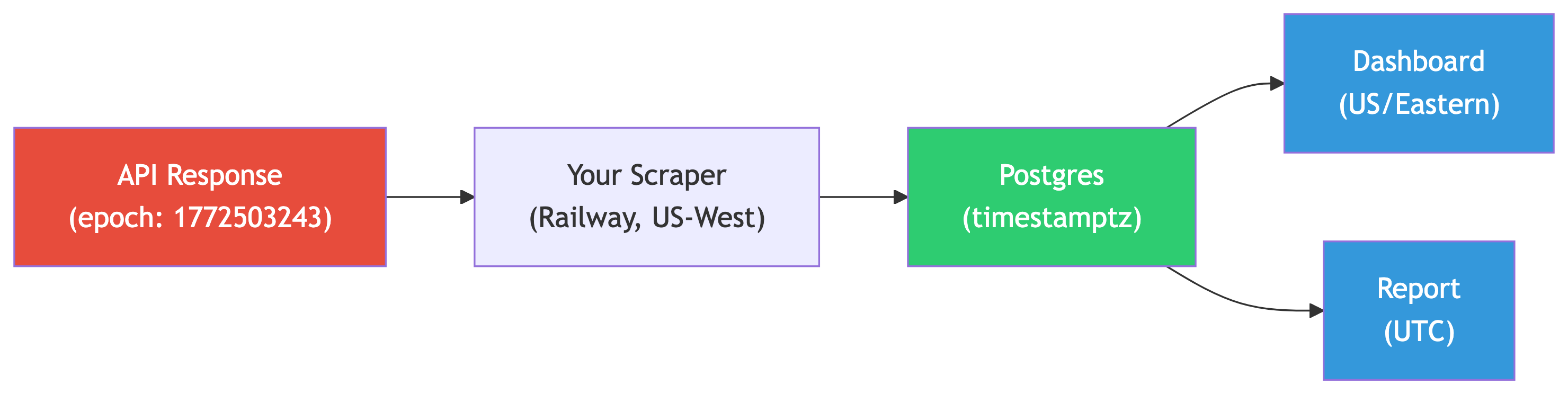
Consider your Railway scrapers. The API returns Unix epoch timestamps (UTC). Your Railway Postgres might be in US/West. Your local Postgres for analysis might be in US/Pacific.

If every column uses timestamptz, this chain works seamlessly. PostgreSQL handles the conversions. If any column uses plain timestamp, you get silent drift.

Best Practices for Timestamps in Pipelines

1. Always use timestamptz for storage
2. Store raw epoch values alongside human-readable timestamps when ingesting API data
3. Set session time zone explicitly at the start of every script
4. Convert at the display layer, not at the storage layer
5. Document your convention in your pipeline README

Part 6: Date and Time Math

You can do arithmetic with dates and times, and it actually makes sense.

Calculations with Dates

Subtracting Dates

Subtract one date from another and you get an integer (days between them):

SELECT '1929-09-30'::date - '1929-09-27'::date;

Result: 3. Three days between September 27 and September 30, 1929.

Adding Intervals

Add an interval to a date:

SELECT '1929-09-30'::date + '5 years'::interval;

Result: 1934-09-30 00:00:00. PostgreSQL handles leap years, month lengths, and calendar quirks automatically.

Subtracting Timestamps

Subtract two timestamps and you get an interval:

SELECT
    '2026-03-18 17:00:00 US/Eastern'::timestamptz -
    '2026-03-18 09:00:00 US/Eastern'::timestamptz
    AS work_day_length;

Result: 08:00:00.

Getting Duration in Specific Units

When you need duration as a number (not an interval), extract the epoch:

SELECT
    EXTRACT(EPOCH FROM (
        '2026-03-18 17:00:00 US/Eastern'::timestamptz -
        '2026-03-18 09:00:00 US/Eastern'::timestamptz
    )) / 3600 AS hours;

Result: 8. This pattern – subtract timestamps, extract epoch, divide – is how you compute durations in minutes, hours, or days as plain numbers. Essential for aggregations and comparisons.

Try It: How Old Is PostgreSQL?

PostgreSQL’s first release was on July 8, 1996. Write a query calculating how many days ago that was.

-- Your query here

SELECT current_date - '1996-07-08'::date AS days_since_postgres;

Part 7: NYC Taxi Trip Analysis

Time to put all of this to work on real data. We have 368,774 taxi rides from June 1, 2016, in New York City.

Patterns in Pickup Times

The Busiest Hours

When do New Yorkers take the most taxi rides?

SET TIME ZONE 'US/Eastern';

SELECT
    date_part('hour', tpep_pickup_datetime) AS trip_hour,
    count(*)
FROM nyc_yellow_taxi_trips
GROUP BY trip_hour
ORDER BY trip_hour;

Run this now. You should get 24 rows.

The busiest hours are in the evening (6 PM to 10 PM). The slowest are early morning (2 AM to 5 AM). The evening peak reflects commutes and nightlife on a summer Wednesday.

Try It: Busiest Hour

Write a query to find the single busiest hour and its trip count.

-- Your query here

SELECT
    date_part('hour', tpep_pickup_datetime) AS trip_hour,
    count(*) AS num_trips
FROM nyc_yellow_taxi_trips
GROUP BY trip_hour
ORDER BY num_trips DESC
LIMIT 1;

Trip Duration Analysis

Median Trip Time by Hour

How long do taxi rides take at different times of day?

SELECT
    date_part('hour', tpep_pickup_datetime) AS trip_hour,
    percentile_cont(.5)
        WITHIN GROUP (ORDER BY
            tpep_dropoff_datetime - tpep_pickup_datetime) AS median_trip
FROM nyc_yellow_taxi_trips
GROUP BY trip_hour
ORDER BY trip_hour;

The longest median trips are around midday (~15 minutes at 1 PM). The shortest are early morning (~8 minutes at 5 AM). Traffic matters.

Try It: The Longest Rides

Find the 10 longest taxi rides by duration. Include pickup time, dropoff time, calculated duration, and trip distance.

Do any results look suspicious?

-- Your query here

SELECT
    tpep_pickup_datetime,
    tpep_dropoff_datetime,
    tpep_dropoff_datetime - tpep_pickup_datetime AS duration,
    trip_distance
FROM nyc_yellow_taxi_trips
ORDER BY duration DESC
LIMIT 10;

You will see rides lasting 20+ hours with zero distance. Data quality issues. The meter was left running, or timestamps were recorded incorrectly.

This is why data engineers never trust raw data. Always profile. Always validate.

Try It: Average Fare by Hour

Write a query showing the average total_amount for each hour. Which hour has the highest average fare?

-- Your query here

SELECT
    date_part('hour', tpep_pickup_datetime) AS trip_hour,
    round(avg(total_amount), 2) AS avg_fare
FROM nyc_yellow_taxi_trips
GROUP BY trip_hour
ORDER BY avg_fare DESC;

Early morning hours (4-5 AM) have the highest average fares. Fewer but longer rides – airport runs and long distances with no traffic.

Time-Series Aggregation with date_trunc

Hourly Rollups

In data engineering, you frequently need to aggregate time-series data into fixed buckets. This is the basis of every dashboard and monitoring system.

SELECT
    date_trunc('hour', tpep_pickup_datetime) AS pickup_hour,
    count(*) AS trips,
    round(avg(total_amount), 2) AS avg_fare
FROM nyc_yellow_taxi_trips
GROUP BY pickup_hour
ORDER BY pickup_hour;

Unlike date_part('hour', ...) which gives you just the number 0-23, date_trunc preserves the full timestamp truncated to the hour. This matters when you have multi-day data – hour 14 on Monday is different from hour 14 on Tuesday.

Try It: Daily Revenue

Write a query using date_trunc to calculate total daily revenue (total_amount). Since this dataset is one day, you should get a single row.

-- Your query here

SELECT
    date_trunc('day', tpep_pickup_datetime) AS trip_date,
    round(sum(total_amount), 2) AS daily_revenue,
    count(*) AS total_trips
FROM nyc_yellow_taxi_trips
GROUP BY trip_date;

Generating Time Series with generate_series

Filling in Missing Time Slots

Real-world time-series data has gaps. If no trips happened at 3:17 AM, that minute is simply absent from your results. Dashboards hate gaps. Pipeline consumers hate gaps.

generate_series creates a continuous sequence of timestamps:

SELECT generate_series(
    '2016-06-01 00:00:00 US/Eastern'::timestamptz,
    '2016-06-01 23:00:00 US/Eastern'::timestamptz,
    '1 hour'::interval
) AS hour_slot;

This produces 24 rows, one for each hour, regardless of whether any trips happened.

Joining with Generated Series

To get a complete hourly report (with zeros for empty hours):

WITH hours AS (
    SELECT generate_series(
        '2016-06-01 00:00:00 US/Eastern'::timestamptz,
        '2016-06-01 23:00:00 US/Eastern'::timestamptz,
        '1 hour'::interval
    ) AS hour_slot
)
SELECT
    h.hour_slot,
    coalesce(count(t.trip_id), 0) AS trip_count
FROM hours h
LEFT JOIN nyc_yellow_taxi_trips t
    ON date_trunc('hour', t.tpep_pickup_datetime) = h.hour_slot
GROUP BY h.hour_slot
ORDER BY h.hour_slot;

This pattern – generate a time spine, left join your data – is fundamental to building reliable time-series reports. You will see it in every analytics platform.

Part 8: Amtrak Train Trips

Let us switch from taxis to trains and watch timestamps cross time zones.

Building the Train Data

Creating and Loading the Table

CREATE TABLE train_rides (
    trip_id bigint GENERATED ALWAYS AS IDENTITY PRIMARY KEY,
    segment text NOT NULL,
    departure timestamptz NOT NULL,
    arrival timestamptz NOT NULL
);

INSERT INTO train_rides (segment, departure, arrival)
VALUES
    ('Chicago to New York',
        '2020-11-13 21:30 CST', '2020-11-14 18:23 EST'),
    ('New York to New Orleans',
        '2020-11-15 14:15 EST', '2020-11-16 19:32 CST'),
    ('New Orleans to Los Angeles',
        '2020-11-17 13:45 CST', '2020-11-18 9:00 PST'),
    ('Los Angeles to San Francisco',
        '2020-11-19 10:10 PST', '2020-11-19 21:24 PST'),
    ('San Francisco to Denver',
        '2020-11-20 9:10 PST',  '2020-11-21 18:38 MST'),
    ('Denver to Chicago',
        '2020-11-22 19:10 MST', '2020-11-23 14:50 CST');

Notice how each timestamp includes the time zone of the city. The subtraction handles cross-zone arithmetic automatically because we used timestamptz.

Calculating Trip Durations

Segment Duration

SELECT segment,
       to_char(departure, 'YYYY-MM-DD HH12:MI a.m. TZ') AS departure,
       arrival - departure AS segment_duration
FROM train_rides;

Two things to notice:

1. to_char() formats timestamps into human-readable strings
2. Subtracting timestamps gives intervals. PostgreSQL correctly handles the time zone differences across segments

Try It: Longest Segment

Which segment takes the longest?

-- Your query here

SELECT segment,
       arrival - departure AS segment_duration
FROM train_rides
ORDER BY segment_duration DESC
LIMIT 1;

San Francisco to Denver: over 32 hours.

Cumulative Trip Duration

Running Total with Window Functions

How long has the entire trip taken after each segment?

SELECT segment,
       arrival - departure AS segment_duration,
       sum(arrival - departure) OVER (ORDER BY trip_id) AS cume_duration
FROM train_rides;

The output shows things like 2 days 85:47:00. PostgreSQL sums the days and hours separately without rolling up.

Fixing with justify_interval()

SELECT segment,
       arrival - departure AS segment_duration,
       justify_interval(sum(arrival - departure)
                        OVER (ORDER BY trip_id)) AS cume_duration
FROM train_rides;

Now the final row shows 5 days 13:47:00. Five and a half days coast to coast by train.

Try It: Format the Output

Rewrite the query with the departure formatted as Mon DD, YYYY HH12:MI AM TZ using to_char().

-- Your query here

SET TIME ZONE 'US/Central';

SELECT segment,
       to_char(departure, 'Mon DD, YYYY HH12:MI AM TZ') AS departure,
       arrival - departure AS segment_duration,
       justify_interval(sum(arrival - departure)
                        OVER (ORDER BY trip_id)) AS cume_duration
FROM train_rides;

Part 9: CTEs and Useful PostgreSQL Features

Complex temporal queries get messy fast. CTEs and a few other PostgreSQL features make them manageable.

Common Table Expressions (CTEs)

What Is a CTE?

A Common Table Expression (CTE) is a temporary, named result set defined with WITH that exists only for the duration of a single query. Think of it as a named intermediate table.

WITH hourly_stats AS (
    SELECT
        date_part('hour', tpep_pickup_datetime) AS trip_hour,
        count(*) AS num_trips,
        round(avg(total_amount), 2) AS avg_fare
    FROM nyc_yellow_taxi_trips
    GROUP BY trip_hour
)
SELECT
    trip_hour,
    num_trips,
    avg_fare
FROM hourly_stats
WHERE num_trips > 10000
ORDER BY trip_hour;

The WITH clause defines hourly_stats. The main query references it like a table. When the query finishes, hourly_stats disappears.

CTEs vs. Subqueries

The equivalent subquery version:

SELECT trip_hour, num_trips, avg_fare
FROM (
    SELECT
        date_part('hour', tpep_pickup_datetime) AS trip_hour,
        count(*) AS num_trips,
        round(avg(total_amount), 2) AS avg_fare
    FROM nyc_yellow_taxi_trips
    GROUP BY trip_hour
) AS hourly_stats
WHERE num_trips > 10000
ORDER BY trip_hour;

Same result. But CTEs are:

• More readable. Logic flows top-to-bottom, not inside-out.
• Reusable. Reference the same CTE multiple times in one query.
• Chainable. Multiple CTEs can build on each other.
• Self-documenting. Good CTE names describe the data at each stage.

In data engineering, CTEs mirror the stages of a transformation pipeline. Each CTE is a logical step: extract, clean, aggregate, enrich.

Chaining CTEs: The Pipeline Pattern

You can define multiple CTEs separated by commas. Each one can reference the ones before it:

WITH hourly AS (
    -- Stage 1: Aggregate by hour
    SELECT
        date_part('hour', tpep_pickup_datetime) AS trip_hour,
        count(*) AS num_trips,
        round(avg(total_amount), 2) AS avg_fare,
        round(avg(trip_distance), 2) AS avg_distance
    FROM nyc_yellow_taxi_trips
    GROUP BY trip_hour
),
ranked AS (
    -- Stage 2: Rank hours by popularity
    SELECT
        trip_hour,
        num_trips,
        avg_fare,
        avg_distance,
        rank() OVER (ORDER BY num_trips DESC) AS popularity_rank
    FROM hourly
)
-- Stage 3: Filter to top 5
SELECT *
FROM ranked
WHERE popularity_rank <= 5
ORDER BY popularity_rank;

Each CTE is simple. The chain is complex. This is the same principle behind well-designed ETL: small, testable, composable transformations.

Try It: Busiest vs. Quietest Hours

Using a CTE, find the 3 busiest and 3 quietest hours by trip count. Combine them into one result with UNION ALL.

-- Your query here

WITH hourly AS (
    SELECT
        date_part('hour', tpep_pickup_datetime) AS trip_hour,
        count(*) AS num_trips
    FROM nyc_yellow_taxi_trips
    GROUP BY trip_hour
)
(SELECT trip_hour, num_trips, 'Busiest' AS category
 FROM hourly ORDER BY num_trips DESC LIMIT 3)
UNION ALL
(SELECT trip_hour, num_trips, 'Quietest' AS category
 FROM hourly ORDER BY num_trips ASC LIMIT 3)
ORDER BY category, num_trips DESC;

The CTE is defined once, used twice. Without it, the GROUP BY aggregation would be duplicated in both halves of the UNION ALL.

Useful PostgreSQL Features

COALESCE: Handling NULLs

COALESCE returns the first non-NULL value from its arguments:

SELECT coalesce(passenger_count, 0) AS passengers
FROM nyc_yellow_taxi_trips
LIMIT 5;

This is critical when combining generate_series with LEFT JOIN. Hours with no trips produce NULL counts, and COALESCE(count, 0) fills the gaps with zeros. In pipeline code, you will use COALESCE constantly – any time you join tables that might not match every row.

HAVING: Filtering After Aggregation

WHERE filters rows before grouping. HAVING filters groups after aggregation:

SELECT
    date_part('hour', tpep_pickup_datetime) AS trip_hour,
    count(*) AS num_trips,
    round(avg(total_amount), 2) AS avg_fare
FROM nyc_yellow_taxi_trips
GROUP BY trip_hour
HAVING count(*) > 15000
ORDER BY trip_hour;

This returns only hours with more than 15,000 trips. The count does not exist until after GROUP BY runs, so WHERE cannot filter on it.

FILTER: Conditional Aggregation (PostgreSQL-Specific)

The FILTER clause lets you apply a condition to a specific aggregate without affecting others in the same query:

SELECT
    date_part('hour', tpep_pickup_datetime) AS trip_hour,
    count(*) AS total_trips,
    count(*) FILTER (WHERE payment_type = '1') AS credit_trips,
    count(*) FILTER (WHERE payment_type = '2') AS cash_trips,
    round(
        count(*) FILTER (WHERE payment_type = '1')::numeric
        / count(*)::numeric * 100, 1
    ) AS credit_pct
FROM nyc_yellow_taxi_trips
GROUP BY trip_hour
ORDER BY trip_hour;

Without FILTER, you would need SUM(CASE WHEN ... THEN 1 ELSE 0 END) for each conditional count. FILTER is cleaner. It is PostgreSQL-specific (not in the SQL standard), but most modern databases have equivalents.

Try It: Tipping Patterns by Hour

Using FILTER, write a query that shows for each hour: the total number of trips, the number of trips that included a tip (tip_amount > 0), and the tipping percentage. Which hours have the highest tipping rates?

-- Your query here

SELECT
    date_part('hour', tpep_pickup_datetime) AS trip_hour,
    count(*) AS total_trips,
    count(*) FILTER (WHERE tip_amount > 0) AS tipped_trips,
    round(
        count(*) FILTER (WHERE tip_amount > 0)::numeric
        / count(*)::numeric * 100, 1
    ) AS tip_pct
FROM nyc_yellow_taxi_trips
GROUP BY trip_hour
ORDER BY tip_pct DESC;

CTE + Date Functions: A Real Pattern

Combining CTEs with temporal analysis is where things get powerful. Here we compute each hour’s trip count, then compare it to the overall average:

WITH hourly_counts AS (
    SELECT
        date_part('hour', tpep_pickup_datetime) AS trip_hour,
        count(*) AS num_trips
    FROM nyc_yellow_taxi_trips
    GROUP BY trip_hour
),
overall AS (
    SELECT round(avg(num_trips), 0) AS avg_hourly_trips
    FROM hourly_counts
)
SELECT
    h.trip_hour,
    h.num_trips,
    o.avg_hourly_trips,
    CASE
        WHEN h.num_trips > o.avg_hourly_trips THEN 'Above Average'
        WHEN h.num_trips < o.avg_hourly_trips THEN 'Below Average'
        ELSE 'Average'
    END AS comparison
FROM hourly_counts h
CROSS JOIN overall o
ORDER BY h.trip_hour;

CTE 1 aggregates by hour. CTE 2 computes the average across all hours. The main query joins them with CROSS JOIN (since overall is a single row) and classifies each hour.

This pattern – aggregate, compute a benchmark, compare – is the backbone of anomaly detection in data pipelines. Is this hour’s traffic normal? Is this day’s revenue within expected range? Same structure, different data.

Try It: Revenue Anomaly Detection

Using two CTEs, find the hours where total revenue is more than one standard deviation above or below the hourly average. Show the hour, its revenue, the average, the standard deviation, and label each as ‘High’, ‘Low’, or ‘Normal’.

Hint: use stddev() alongside avg() in the second CTE.

-- Your query here

WITH hourly_revenue AS (
    SELECT
        date_part('hour', tpep_pickup_datetime) AS trip_hour,
        round(sum(total_amount), 2) AS hour_revenue
    FROM nyc_yellow_taxi_trips
    GROUP BY trip_hour
),
stats AS (
    SELECT
        round(avg(hour_revenue), 2) AS avg_revenue,
        round(stddev(hour_revenue), 2) AS stddev_revenue
    FROM hourly_revenue
)
SELECT
    h.trip_hour,
    h.hour_revenue,
    s.avg_revenue,
    s.stddev_revenue,
    CASE
        WHEN h.hour_revenue > s.avg_revenue + s.stddev_revenue THEN 'High'
        WHEN h.hour_revenue < s.avg_revenue - s.stddev_revenue THEN 'Low'
        ELSE 'Normal'
    END AS anomaly_label
FROM hourly_revenue h
CROSS JOIN stats s
ORDER BY h.trip_hour;

Part 10: Putting It All Together (Exercises)

Let’s combine several concepts from today into more complex queries.

Combined Exercises

Try It: Taxi Trips by Day of Week

Count trips by day of the week using a CASE statement for day names:

-- Your query here

SET TIME ZONE 'US/Eastern';

SELECT
    CASE date_part('dow', tpep_pickup_datetime)
        WHEN 0 THEN 'Sunday'
        WHEN 1 THEN 'Monday'
        WHEN 2 THEN 'Tuesday'
        WHEN 3 THEN 'Wednesday'
        WHEN 4 THEN 'Thursday'
        WHEN 5 THEN 'Friday'
        WHEN 6 THEN 'Saturday'
    END AS day_name,
    count(*) AS num_trips
FROM nyc_yellow_taxi_trips
GROUP BY day_name
ORDER BY num_trips DESC;

Since this dataset is from June 1, 2016 (a Wednesday), only one row appears. But the pattern works on multi-day datasets.

Try It: Time Zone Conversion

Show the first 5 taxi pickup times converted to Asia/Tokyo time.

-- Your query here

SELECT
    tpep_pickup_datetime AS nyc_time,
    tpep_pickup_datetime AT TIME ZONE 'Asia/Tokyo' AS tokyo_time
FROM nyc_yellow_taxi_trips
ORDER BY tpep_pickup_datetime
LIMIT 5;

Tokyo is 13 hours ahead of New York in summer. A 9 PM Wednesday pickup in NYC is 10 AM Thursday in Tokyo.

Try It: Trip Duration Percentiles

Calculate the 25th, 50th (median), and 75th percentile of trip duration:

-- Your query here

SELECT
    percentile_cont(0.25)
        WITHIN GROUP (ORDER BY tpep_dropoff_datetime - tpep_pickup_datetime)
        AS p25,
    percentile_cont(0.50)
        WITHIN GROUP (ORDER BY tpep_dropoff_datetime - tpep_pickup_datetime)
        AS median,
    percentile_cont(0.75)
        WITHIN GROUP (ORDER BY tpep_dropoff_datetime - tpep_pickup_datetime)
        AS p75
FROM nyc_yellow_taxi_trips;

The IQR (P75 - P25) tells you how spread out typical trips are.

Try It: Correlation Challenge

Calculate the correlation coefficient between trip duration (in seconds) and total_amount. Then do the same for trip_distance and total_amount. Limit to rides of 3 hours or less.

Which is a better predictor of fare: time or distance?

-- Your query here

SELECT
    round(
        corr(
            date_part('epoch', tpep_dropoff_datetime - tpep_pickup_datetime),
            total_amount
        )::numeric, 4
    ) AS duration_fare_corr,
    round(
        corr(trip_distance, total_amount)::numeric, 4
    ) AS distance_fare_corr
FROM nyc_yellow_taxi_trips
WHERE tpep_dropoff_datetime - tpep_pickup_datetime <= '3 hours'::interval;

Distance correlates more strongly with fare. NYC taxi meters are primarily distance-based.

Part 11: What We Learned

Summary

Key Concepts

Concept	What It Does
timestamptz	The go-to type for storing moments in time
date_part() / extract()	Pull year, month, hour, etc. from a timestamp
date_trunc()	Round timestamps down to a precision (essential for time-series)
make_timestamptz()	Build timestamps from components
current_timestamp / now()	Time when the query started
clock_timestamp()	Actual clock time (changes per row)
SET TIME ZONE	Change display for your session
AT TIME ZONE	One-off conversion to another zone
to_char()	Format timestamps as readable strings
justify_interval()	Clean up messy interval output
generate_series()	Create continuous time spines for gap-free reporting
WITH (CTE)	Define named temporary result sets; mirrors pipeline stages
COALESCE	Return the first non-NULL value (essential for outer joins)
HAVING	Filter groups after aggregation
FILTER (WHERE ...)	Apply conditions to individual aggregates (PostgreSQL-specific)

The Big Ideas

1. Always use timestamptz. A timestamp without a zone is a bug waiting to happen.
2. Time zones change the display, not the data. PostgreSQL stores everything as UTC.
3. Subtracting timestamps gives you intervals. That is how you calculate durations.
4. CTEs mirror pipeline stages. Each CTE is a named, testable transformation step.
5. date_trunc is your best friend for time-series aggregation in pipelines.
6. Generate time spines with generate_series to fill gaps in your data.
7. Use FILTER for conditional aggregation. Cleaner than SUM(CASE ...) when you need multiple conditional counts or sums.
8. Real-world data is messy. Always sanity-check your results.

References

1. DeBarros, A. (2022). Practical SQL: A Beginner’s Guide to Storytelling with Data (2nd ed.). No Starch Press. Chapter 12.
2. PostgreSQL Date/Time Functions: https://www.postgresql.org/docs/current/functions-datetime.html
3. PostgreSQL Formatting Functions: https://www.postgresql.org/docs/current/functions-formatting.html
4. NYC TLC Trip Record Data: https://www.nyc.gov/site/tlc/about/tlc-trip-record-data.page
5. ISO 8601 Date and Time Standard: https://en.wikipedia.org/wiki/ISO_8601